CARLA; Self-supervised Contrastive Representation Learning for Time Series Anomaly Detection

CARLA: Self-supervised Contrastive Representation Learning for Time Series Anomaly Detection

https://arxiv.org/pdf/2306.15489

Contents

1. Abstract
2. Introduction
3. CARLA
   1. Overview
   2. Problem Definition
   3. Stage 1: Pretext Stage
   4. Stage 2: Self-supervised Classficaiton Stage
   5. Inference
4. Experiments

Abstract

CARLA = CL for TSAD

Existing CL methods

• Assume that augmented TS windows are positive samples
• Assume that temporally distant TS windows are negative samples

\(\rightarrow\) Argue that these assumptions are limited!!!

\(\because\) Augmentation can transform them to negative samples!

1. Introduction

Contribution

• [1] Novel CL model to detect anomalies in TS
  • Both UTS & MTS
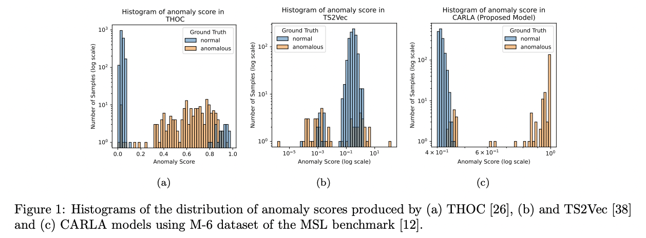
  • Learns to effectively discriminate anomalous ones in the feature space
  • Code: https: //github.com/zamanzadeh/CARLA
• [2] Effective CL method for TSAD
  • To learn feature representations for a pretext task
    • By leveraging existing generic knowledge about TS anomalies
• [3] Self-supervised classification method
  • Classify TS windows
  • Goal: Classify each sample by utilising its neighbours in the representation space
    • Representation space: Learned in the pretext stage
• [4] Experiments
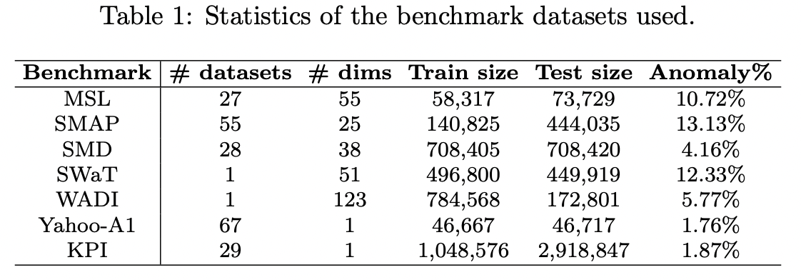
  • Seven real-world benchmark datasets
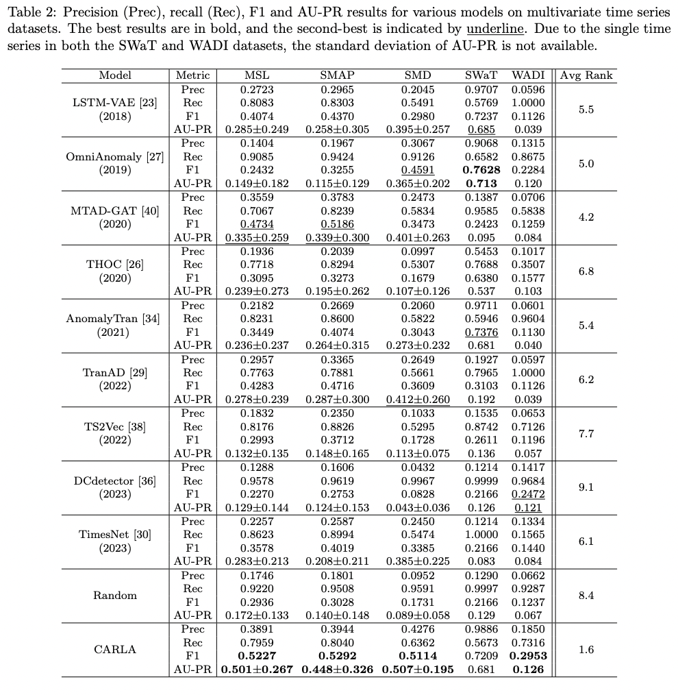
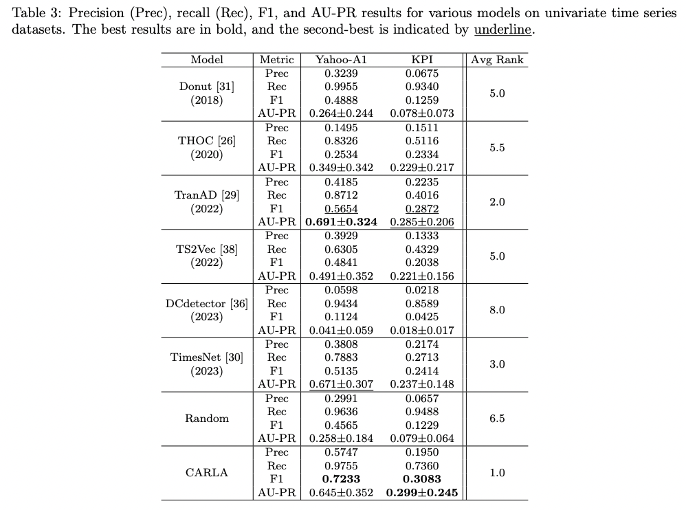
  • vs. 10 SOTA unsupervised, semi-supervised, and self-supervised contrastive learning models.

2. CARLA

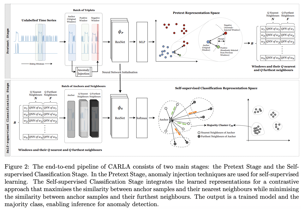
(1) Overview

(2) Problem Definition

Time series \(\mathcal{D}\) : Partitioned into \(m\) overlapping windows \(\left\{w_1, \ldots, w_i, \ldots, w_m\right\}\)

• with stride 1 where \(w_i=\left\{x_1, \ldots, x_i, \ldots, x_{W S}\right\}\),
• WS = TS window size
• \[x_i \in \mathbb{R}^{\text {Dim }}\]

CARLA: Built on several key components

Consists of two main stages

• Stage 1) Pretext Stage

• Stage 2) Self-supervised Classification Stage.

(3) Stage 1: Pretext Stage

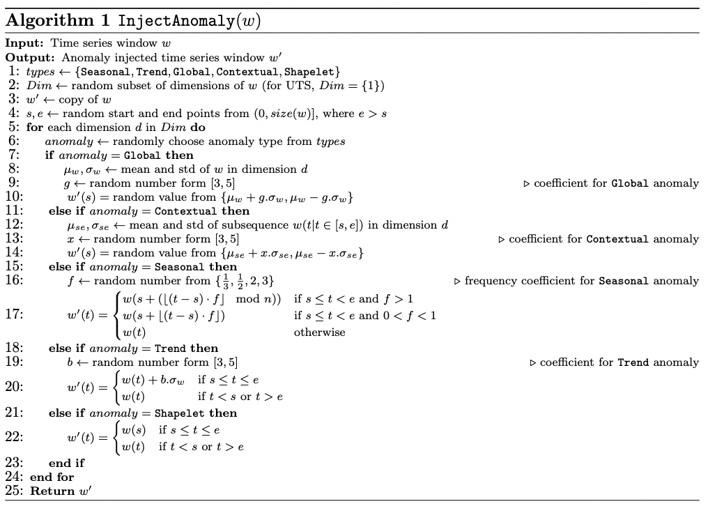
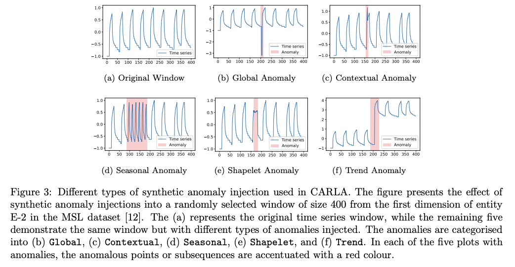
Employs anomaly injection: To learn ..

• (1) Similar representations for temporally proximate windows
• (2) Distinct representations for anomalous windows

Anomaly injection

Stage 1-1) Contrastive Representation Learning

• \(\mathcal{L}_{\text {Pretext }}\left(\phi_p, \mathcal{T}, \alpha\right)=\frac{1}{\mid \mathcal{T}\mid } \sum_{(\alpha, p, n) \in \mathcal{T}} \max \left(\mid \phi_p(a)-\phi_p(p)\mid _2^2-\mid \phi_p(a)-\phi_p(n)\mid _2^2+\alpha, 0\right)\).

Stage 1-2) Nearest and Furtherest Neighbours

• For each sample, identify semantically meaningful nearest & furthest neighbours
• Based on the representation space obtained in Stage 1-1)

Pseudocode

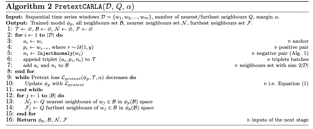
Result: Establish a prior by finding the nearest and furthest neighbours for each window representation for the next stage!

(4) Stage 2: Self-supervised Classification Stage

Classifies these window representations as normal or anomalous!

\(\rightarrow\) Based on the proximity of their neighbours in the representation space

Notation

• Classes \(\mathcal{C}=\{1, \ldots, C\}\)
• Model \(\phi_s(w) \in[0,1]^c\).

**Pairwise similarity **

• Between the probability distributions of the anchor and its neighbours

• \(\text { similarity }\left(\phi_s, w_i, w_j\right)=\left\langle\phi_s\left(w_i\right) \cdot \phi_s\left(w_j\right)\right\rangle=\phi_s\left(w_i\right)^{\top} \phi_s\left(w_j\right)\).

Loss 1) Consistency loss

• Binary CE loss

• Maximise the similarity between the anchor and nearest neighbours

• \(\mathcal{L}_{\text {consistency }}\left(\phi_s, \mathcal{B}, \mathcal{N}\right)=-\frac{1}{\mid \mathcal{B}\mid } \sum_{w \in \mathcal{B}} \sum_{w_s \in \mathcal{N}_w} \log \left(\text { similarity }\left(\phi_s, w, w_n\right)\right)\).

Loss 2) Inconsistency loss

• \(\mathcal{L}_{\text {inconsistency }}\left(\phi_s, \mathcal{B}, \mathcal{F}\right)=-\frac{1}{\mid \mathcal{B}\mid } \sum_{w \in \mathcal{B}} \sum_{w_n \in \mathcal{F}_w} \log \left(\operatorname{similarity}\left(\phi_s, w, w_n\right)\right)\).

Loss 3) Entropy loss

• To encourage class diversity and prevent overfitting
• Entropy on the distribution of anchor and neighbour samples across classes.
• \(\mathcal{L}_{\text {entropy }}\left(\phi_s, \mathcal{B}, \mathcal{C}\right)=\sum_{c \in \mathcal{C}} \dot{\phi}_g \log \left(\dot{\phi}_g\right) \text { where } \dot{\phi}_g^c=\frac{1}{\mid \mathcal{B}\mid } \sum_{w_i \in \mathcal{B}} \phi_g^c\left(w_i\right)\).
  • \(\phi_s^c\left(w_i\right)\): Probability of window \(w_i\) being assigned to class \(c\)

Final loss function:

\(\begin{aligned} & \mathcal{C}_{\text {Sedf-mpervised }}\left(\phi_{,}, B, N, \mathcal{F}, \mathcal{C}, \beta\right)= \\ & \mathcal{L}_{\text {emsustency }}\left(\phi_n, \mathcal{B}, \mathcal{N}\right)-\mathcal{L}_{\text {internstatery }}\left(\phi_n, \mathcal{B}, \mathcal{F}\right)-\beta \cdot \mathcal{L}_{\text {entropy }}\left(\phi_n, \mathcal{B}, C\right) \end{aligned}\).

Pseudocode

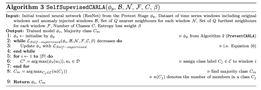
(5) Inference

Determine the class assignments for set \(\mathcal{D}\) and majority class \(C_{\mathrm{m}}\),

\(\rightarrow\) \(C_{\mathrm{m}}=\arg \max _{C_j \in c}\left(n\left(C_j\right)\right)\)

For every new window \(w_i\) …

• Calculate \(\phi_0^{C-}\left(w_t\right)\)
  • Probability of \(w_T\) being assigned to the majority class \(C_m\).
• Class \(w_l\) as normal / anomalous based on whether it belongs to the majority class

Anomaly label & score

\(\text { Anomaly label }\left(w_i\right): \begin{cases}0, & \text { if } \forall c \in \mathcal{C}, \phi_i^C=m\left(w_i\right) \geq \phi_i^C\left(w_i\right) \\ 1, & \text { otherwise }\end{cases}\).

\(\text { Anomaly score }\left(w_t\right)=1-\phi_g^{C-}\left(w_t\right)\).

3. Experiments