(paper) Unsupervised Representation Learning for TS with Temporal Neighborhood Coding

Unsupervised Representation Learning for TS with Temporal Neighborhood Coding (2021, 14)

Contents

1. Abstract
2. Introduction
3. Method

0. Abstract

Time Series : sparsely labeled

\(\rightarrow\) propose a SELF-supervised framework, for learning representation for non-stationary TS

TCN (Temporal Neighborhood Coding)

• distribution of signals from within NEIGHBORHOOD

  is distinguishable from the distribution of NON-neighborhood signals

1. Introduction

Unsupervised Representaiton Learning

• extract informative LOW-dim representaiton from raw TS,

  by leveraging the data’s inherent structure

Requirements

• (1) need to be efficient and scalable

• (2) should acount for & able to model dynamic changes that occur wihtin samples

  ( i.e non-stationarity )

This paper proposes “TCN”

• self-supervised framework for learning representations for complex MULTIVARIATE NON-stationary TS

• setting : latent distn of signals CHANGES OVER TIME

  \(\rightarrow\) aims to capture the progression of underlying temporal dynamics

• characteristics
  • (1) efficient
  • (2) scalable to high-dim
  • (3) can be used in different TS settings
• transferable to many downstream tasks

2. Method

• encode the underlying state of multivariate, non-stationary TS

• takes advantage of local smoothness of the generative process of signals

Notation

• \(X \in R^{D \times T}\) : MTS

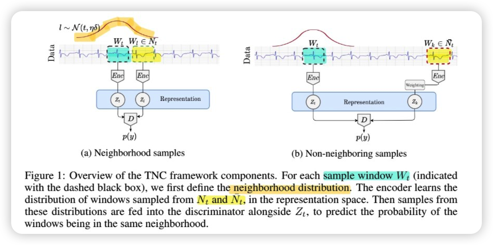
• \(X_{\left[t-\frac{\delta}{2}, t+\frac{\delta}{2}\right]}\) : window ……. refer as \(W_t\)

• \(N_t\) : temporal neighborhood of window \(W_t\)

  • set of all windows, with centroids \(t^{*}\), where \(t^{* } \sim N(t, \eta \cdot \delta)\)
    • \(\eta\) : range of neighborhood
  • how to set \(\eta\) ?
    • (1) domain experts
    • (2) determined by analyzing the stationarity properties of the signal for every \(W_t\)

• \(\bar{N_t}\) : non-neighborhood of window \(W_t\)

  ( considered as negative samples )

since nieghborhood represents similar samples,

• range should identify the approximate time span within which the signal remains stationarity & the generative process does not change

• use ADF test (Augmented Dickey-Fuller test to determine the region for every window

Value of \(\eta\)

• too SMALL : many samples within neighborhood will OVERLAP

• too BIG : the neighborhood would span over multiple ounderlying states

  ( fail to distinguish among these states )

Sampling bias

• occurs, because randomly drawing negative samples from data distn may result in negative samples, that are actually SIMILAR to the reference
  • ex) far away from \(W_t\) ( = non-neighborhood ), but may be similar to reference

\(\rightarrow\) solution : consider samples from \(\bar{N_t}\) As…

• Unlabeled samples (O)
• Negative samples (X)

( idea from Positive-Unlabeled Learning )

PU Learning

classifier is learned using…

• (1) positive samples (P)
• (2) unlabeled data (U)
  • mixture of P & N
  • with a positive classs prior \(\pi\)

PU learning falls into 2 categories

• (1) identify negative samples from the unlabeled cohort
• (2) treat the unlabeled data as negative samples with smaller weights
  • unlabeled samples should be properly weighted to make an unbiased classifier

Samples from…

• (1) neighborhood ( \(N_t\) ) : positive
• (2) non-neighborhood ( \(\bar{N_t}\) ) : combination of positive ( weight : \(w\) ) & negative ( weight : \(1-w\) )
  • weight (\(w\)) : probability of having samples similar to \(W_t\) in \(\bar{N}\)
    • (1) can be approximated using the prior knowledge
    • (2) or tuned as hyperparameter

After defining neighborhood distn…train an objective function

Key point of Encoder :

• preserve the neighborhood properties in the encoding space
• Notation
  • \(Z_l = Enc(W_l)\) ….. where \(W_l \in N_t\)
  • \(Z_k = Enc(W_k)\) ….. where \(W_k \in \bar{N_t}\)

2 main components of TNC

(1) Encoder : \(Z_t = Enc(W_t)\)

• maps \(W_t \in R^{D \times \delta}\) to \(Z_t \in R^{M}\)

(2) Discriminator : \(D(Z_t, Z)\)

• approximates the probability of \(Z\) being the representation of a window in \(N_t\)
• predicts the probability of samples belonging to the same temporal neighborhood
• details
  • use a simple multi-headed binary classifier

Objective Function

\[\begin{gathered} \mathcal{L}=-\mathbb{E}_{W_{t} \sim X}\left[\mathbb{E}_{W_{l} \sim N_{t}}[\log \underbrace{\mathcal{D}\left(\operatorname{Enc}\left(W_{t}\right), \operatorname{Enc}\left(W_{l}\right)\right)}_{\mathcal{D}\left(Z_{t}, Z_{l}\right)}+\mathbb{E}_{W_{k} \sim \bar{N}_{t}}[\left(1-w_{t}\right) \times \log \underbrace{\left(1-\mathcal{D}\left(Z_{t}, Z_{k}\right)\right)}_{\mathcal{D}\left(\operatorname{Enc}\left(W_{t}\right), \operatorname{Enc}\left(W_{k}\right)\right)}+w_{t} \times \log \mathcal{D}\left(Z_{t}, Z_{k}\right)]]\right]. \end{gathered}\]