Time Series as Images; Vision Transformer for Irregularly Sampled Time Series

Time Series as Images: Vision Transformer for Irregularly Sampled Time Series

Contents

Abstract

Irregular sampled time series (= ITS)

• Complex dynamics
• Pronounced sparsity

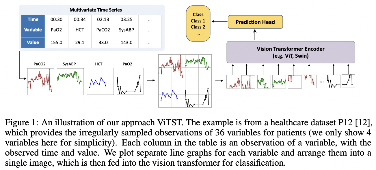
ViTST

• Idea) Convert ITS $\rightarrow$ line graph images
• Model) Pretrained ViT
• Task) TS classification
• Potential to serve as a universal framework for TS modeling
• Experiments
  • SoTA on healthcare and human activity datasets
    • e.g., leave-sensors-out setting
      • where a portion of variables is omitted during testing
  • Strong at missing observations
• Code) https://github.com/Leezekun/ViTST

1. Introduction

Research Question

Can these powerful pre-trained vision transformers capture temporal patterns in visualized time series data, similar to how humans do?

Proposal: ViTST (Vision Time Series Transformer)

• (1) IMTS to line graph
  • Into a standard RGB image
• (2) Finetune a pre-trained vViT

Line graphs

• Effective and efficient visualization technique for TS
• Capture crucial patterns
  • e.g., temporal dynamics (represented within individual line graphs)
  • e.g., interrelations between variables (throughout separate graphs)

Experiments

• Superior performance over SoTA designed for ITS
• Exceeded prior SoTA
  • Dataset = P19 & P12
    • (AUROC) 2.2% & 0.7%
    • (AUPRC) 1.3% & 2.9%
  • Dataset = PAM (human activity)
    • (Acc, Precision, Recall, F1) 7.3%, 6.3%, 6.2%, 6.7%
• Srong robustness to missing observations

Contributions

1. Simple yet highly effective approach for IMTS classification
2. Excellent results on both irregular and regular TS
3. Successful transfer of knowledge from pretrained ViT to TS

2. Related Works

(1) Irregularly sampled time series

Definition) Sequence of observations with varying time intervals

• IMTS: Different variables within the 2 same time series may not align

Common approach

• Convert continuous-time observations into fixed time intervals

a) Non-attention based

• (1) GRU-D: Decays the hidden states based on gated recurrent units (GRU)
• (2) Multi-directional RNN: Capture the inter- and intra-steam patterns

b) Attention based

• ATTAIN: Attention + LSTM to model time irregularity
• SeFT: Maps the ITS into a set of observations based on differentiable set functions
• mTAND: Learns continuous-time embeddings
  • With a multi-time attention mechanism
• UTDE: Integrates embeddings from mTAND and classical imputed TS with learnable gates
• Raindrop: Models irregularly sampled time series as graphs
  • Utilizes GNN

(2) Imaging time series

• Gramian fields [39], recurring plots [14, 37], and Markov transition fields [40]
• Typically employ CNNs
  • Limitation: Often require domain expertise

3. Approach

(1) Overview

a) Two steps

• Step 1) Transforming IMTS to line graph
• Step 2) Employ pre-trained ViT as an image classifier

b) Two components

• (1) Function that transforms the time series $\mathcal{S}_i$ into an image $\mathrm{x}_i$
• (2) Image classifier that takes the line graph image $\mathrm{x}_i$ as input and predicts the label $\hat{y}_i$.

c) Notation

$\mathcal{D}=\left{\left(\mathcal{S}_i, y_i\right) \mid i=1, \cdots, N\right}$: TS dataset with $N$ samples

• (y) $y_i \in{1, \cdots, C}$, where $C$ is the number of classes.

• (X) $\mathcal{S}_i$ consists of observations of $D$ variables at most

  ( = some might have no observations)

Format: $\left[\left(t_1^d, v_1^d\right),\left(t_2^d, v_2^d\right), \cdots,\left(t_{n_d}^d, v_{n_d}^d\right)\right]$

• Observations for each variable $d$ are given by a sequence of tuples with observed time and value

IMTS = Intervals between observation times $\left[t_1^d, t_2^d, \cdots, t_{n_d}^d\right]$ are different across variables or samples

(1) “TS to Image” Transformation

a) Time series line graph

Line graph

• Prevalent method for visualizing temporal data points
• Each point = Observation marked by its time and value
• Horizontal axis = Timestamps
• Vertical axis = Values

. Observations are connected with straight lines in chronological order, with any missing values interpolated seamlessly. This graphing approach allows for flexibility for users in plotting time series as images, intuitively suited for the processing efficiency of vision transformers. The practice mirrors prompt engineering when using language models, where users can understand and adjust natural language prompts to enhance the model performance. In our practice, we use marker symbols “ $*$ “ to indicate the observed data points in the line graph. Since the scales of different variables may vary significantly, we plot the observations of each variable in an individual line graph, as shown in Fig. 1. The scales of each line graph $g_{i, d}$ are kept the same across different time series $\mathcal{S}_i$. We employ distinct colors for each line graph for differentiation. Our initial experiments indicated that tick labels and other graphical components are superfluous, as an observation’s position inherently signals its relative time and value magnitude. We investigated the influences of different choices of time series-to-image transformation in Section 4.3.

b) Image Creation

. Given a set of time series line graphs $\mathcal{G}_i=\mathrm{g}_1, \mathrm{~g}_2, \cdots, \mathrm{~g}_D$ for a time series $\mathcal{S}_i$, we arrange them in a single image $\mathrm{x}_i$ using a pre-defined grid layout. We adopt a square grid by default, following [10]. Specifically, we arrange the $D$ time series line graphs in a grid of size $l \times l$ if $l \times(l-1)<D \leq l \times l$, and a grid of size $l \times(l+1)$ if $l \times l<D \leq l \times(l+1)$. For example, the P19, P12, and PAM datasets contain 34, 36, and 17 variables, respectively, and the corresponding default grid layouts are $6 \times 6,6 \times 6$, and $4 \times 5$. Any grid spaces not occupied by a line graph remain empty. Figure 6 showcases examples of the resulting images. As for the order of variables, we sort them according to the missing ratios for irregularly sampled time series. We explored the effects of different grid layouts and variable orders in Section 4.3.