Predict, Refine, Synthesize; Self-Guiding Diffusion Models for Probabilistic Time Series Forecasting

Predict, Refine, Synthesize: Self-Guiding Diffusion Models for Probabilistic Time Series Forecasting

Contents

1. Abstract

2. Introduction

3. Background
   1. DDPM
   2. Diffusion Guidance
4. TSDiff
   1. Observation Self-Guidance
   2. Prediction Refinement

Abstract

Previous TS diffusion models:

• focused on developing conditional models tailored to specific forecasting or imputation tasks

TSDiff

• TSDiff = Unconditionally-trained diffusion model for time series
• Explore the potential of task-agnostic, unconditional diffusion models
• Self-guidance mechanism
  • Enables conditioning TSDiff for downstream tasks during inference
    • without requiring auxiliary networks or altering the training procedure

3 different TS tasks

• (1) Forecasting
  • competitive with several task-specific conditional forecasting methods (predict)
• (2) Refinement
  • leverage the learned implicit probability density of TSDiff to iteratively refine the predictions of base forecasters with reduced computational overhead over reverse diffusion (refine)
• (3) Synthetic data generation
  • downstream forecasters trained on synthetic samples from TSDiff outperform forecasters that are trained on samples from other SOTA generative time series models

1. Introduction

Diffusion models

• Outstanding performance on generative tasks across various domains

• Use conditional diffusion models for TS forecasting and imputation tasks

  \(\rightarrow\) Task specific …. forego the desirable unconditional generative capabilities of diffusion models.

Question) Can we address multiple (even conditional) downstream tasks with an unconditional diffusion model?

Answer) TSDiff

TSDiff

Unconditional diffusion model for TS

Propose two inference schemes to utilize the model for forecasting.

• (1) Self-guidance mechanism
  • Enables conditioning the model during inference, without requiring auxiliary networks.
  • Makes the unconditional model amenable to arbitrary forecasting (and imputation) tasks
  • Experiment: competitive against task-specific models, without requiring conditional training.
• (2) Method to iteratively refine predictions of base forecasters
  • with reduced computational overhead compared to reverse diffusion
  • interpret the implicit probability density learned by TSDiff as an energy-based prior

Generative capabilities of TSDiff

• Train multiple downstream forecasters on synthetic samples from TSDiff
• Linear Predictive Score (LPS)
  • to quantify the generative performance
  • test forecast performance of a linear ridge regression model trained on synthetic samples.

2. Background

(1) DDPM

pass

(2) Diffusion Guidance

Classifier guidance

• Repurposes unconditionally-trained image diffusion models for class-conditional image generation
• Decompose the class-conditional score function using the Bayes rule
  • \(\nabla_{\mathbf{x}^t} \log p\left(\mathbf{x}^t \mid c\right)=\nabla_{\mathbf{x}^t} \log p\left(\mathbf{x}^t\right)+\nabla_{\mathbf{x}^t} \log p\left(c \mid \mathbf{x}^t\right)\).
• Employing an auxiliary classifier to estimate \(\nabla_{\mathbf{x}^t} \log p\left(c \mid \mathbf{x}^t\right)\).

Modified reverse diffusion process

• allows sampling from the class-conditional distribution,

• \(p_\theta\left(\mathbf{x}^{t-1} \mid \mathbf{x}^t, c\right)=\mathcal{N}\left(\mathbf{x}^{t-1} ; \mu_\theta\left(\mathbf{x}^t, t\right)+s \sigma_t^2 \nabla_{\mathbf{x}^t} \log p\left(c \mid \mathbf{x}^t\right), \sigma_t^2 \mathbf{I}\right)\).

  • \(s\): scale parameter controlling the strength of the guidance.

3. TSDiff: an Unconditional Diffusion Model for Time Series

Problem Statement

Notation

• \(\mathbf{y} \in \mathbb{R}^L\) : TS of length \(L\).
• obs \(\subset\{1, \ldots, L\}\) : set of observed timesteps
• ta : complement set of target timesteps

Goal

• Recover the complete \(\mathbf{y}\), given the observed \(\mathbf{y}_{\mathrm{obs}}\)

  ( Formally, this involves modeling the conditional distribution \(p_\theta\left(\mathbf{y}_{\mathrm{ta}} \mid \mathbf{y}_{\mathrm{obs}}\right)\).

• Seek to train a single unconditional generative model, \(p_\theta(\mathbf{y})\)

  & Condition it during inference to draw samples \(p_\theta\left(\mathbf{y}_{\text {ta }} \mid \mathbf{y}_{\text {obs }}\right)\).

Generative Model Architecture

Begin with modeling the marginal probability, \(p_\theta(\mathbf{y})\), via a diffusion model ( = TSDiff )

Architecture

• Based on SSSD ( modification of DiffWave ) employing S4 layers

• Designed to handle univariate sequences of length \(L\).

• To incorporate historical information beyond \(L\) timesteps without increasing \(L\), we append lagged TS along the channel dimension.

  \(\rightarrow\) Noisy input \(\mathbf{x}^t \in \mathbb{R}^{L \times C}\) to the diffusion model

  • where \(C-1\) is the number of lags.

• (1) S4 layers = operate on time dimension

• (2) Conv1x1 layers = operate on channel dimension

• Output dimensions = Input dimensions
• Can be modified to handle multivariate TS by incorporating additional layers, e.g., a transformer layer, operating across the feature dimensions after the S4 layer

Discuss 2 approaches to condition the generative model, \(p_\theta(\mathbf{y})\), during inference, enabling us to draw samples from \(p_\theta\left(\mathbf{y}_{\text {ta }} \mid \mathbf{y}_{\text {obs }}\right)\).

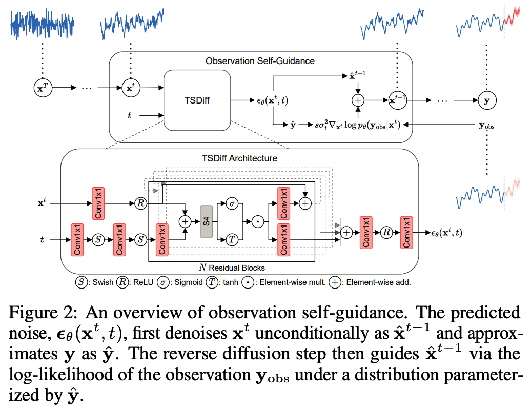
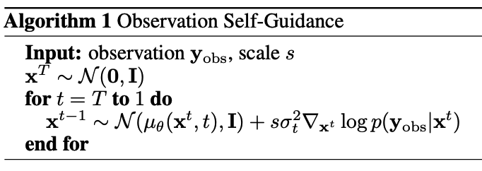
(1) Observation Self-Guidance

\(p_\theta\left(\mathbf{x}^t \mid \mathbf{y}_{\text {obs }}\right) \propto p_\theta\left(\mathbf{y}_{\text {obs }} \mid \mathbf{x}^t\right) p_\theta\left(\mathbf{x}^t\right)\).

• \(t \geq 0\) : Arbitrary diffusion step

\(\nabla_{\mathbf{x}^t} \log p_\theta\left(\mathbf{x}^t \mid \mathbf{y}_{\text {obs }}\right)=\nabla_{\mathbf{x}^t} \log p_\theta\left(\mathbf{y}_{\text {obs }} \mid \mathbf{x}^t\right)+\nabla_{\mathbf{x}^t} \log p_\theta\left(\mathbf{x}^t\right)\).

• with guidance distribution, \(p_\theta\left(\mathbf{y}_{\text {obs }} \mid \mathbf{x}^t\right)\), we can draw samples from \(p_\theta\left(\mathbf{y}_{\text {ta }} \mid \mathbf{y}_{\text {obs }}\right)\)
  • using guided reverse diffusion
  • \(p_\theta\left(\mathbf{x}^{t-1} \mid \mathbf{x}^t, \mathbf{y}_{\text {obs }}\right)=\mathcal{N}\left(\mathbf{x}^{t-1} ; \mu_\theta\left(\mathbf{x}^t, t\right)+s \sigma_t^2 \nabla_{\mathbf{x}^t} \log p_\theta\left(\mathbf{y}_{\text {obs }} \mid \mathbf{x}^t\right), \sigma_t^2 \mathbf{I}\right)\).
• HOWEVER, we do not have access to auxiliary guidance networks

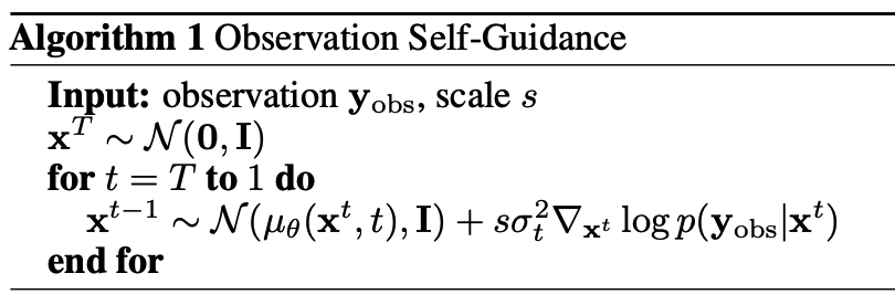
Propose two variants of a self-guidance mechanism

• that utilizes the same diffusion model to parameterize the guidance distribution
• Intuition) model designed for complete sequences should reasonably approximate partial sequences.

a) Mean Square Self-Guidance

Model \(p_\theta\left(\mathbf{y}_{\text {obs }} \mid \mathbf{x}^t\right)\) as a multivariate Gaussian distribution,

• \(p_\theta\left(\mathbf{y}_{\text {obs }} \mid \mathbf{x}^t\right)=\mathcal{N}\left(\mathbf{y}_{\text {obs }} \mid f_\theta\left(\mathbf{x}^t, t\right), \mathbf{I}\right)\)….. Eq (a)

Reuse the denoising network \(\epsilon_\theta\) to estimate \(\mathbf{y}\) :

• \(\hat{\mathbf{y}}=f_\theta\left(\mathbf{x}^t, t\right)=\frac{\mathbf{x}^t-\sqrt{\left(1-\bar{\alpha}_t\right)} \boldsymbol{\epsilon}_\theta\left(\mathbf{x}^t, t\right)}{\sqrt{\bar{\alpha}_t}}\).
  • with \(\epsilon=\epsilon_\theta\left(\mathbf{x}^t, t\right)\) …. one-step denoising
• Requires no auxiliary networks or changes to the training procedure

Logarithm to Eq (a) & drop constant terms

\(\rightarrow\) mean squared error (MSE) loss on the observed part of the TS

• \(\hat{\mathbf{y}}=f_\theta\left(\mathbf{x}^t, t\right)=\frac{\mathbf{x}^t-\sqrt{\left(1-\bar{\alpha}_t\right)} \boldsymbol{\epsilon}_\theta\left(\mathbf{x}^t, t\right)}{\sqrt{\bar{\alpha}_t}}\).

b) Quantile Self-Guidance

Probabilistic forecasts are often evaluated using quantile-based metrics

• ex) cotinuous ranked probability score (CRPS)

MSE vs. CRPS

• MSE: only quantifies the average quadratic deviation from the mean

• CRPS: takes all quantiles of the distribution into account by integrating the quantile loss from 0 to 1

\(\rightarrow\) substitute the Gaussian distribution with the asymmetric Laplace disn

\(p_\theta\left(\mathbf{y}_{\text {obs }} \mid \mathbf{x}^t\right)=\frac{1}{Z} \cdot \exp \left(-\frac{1}{b} \max \left\{\kappa \cdot\left(\mathbf{y}_{\text {obs }}-f_\theta\left(\mathbf{x}^t, t\right)\right),(\kappa-1) \cdot\left(\mathbf{y}_{\text {obs }}-f_\theta\left(\mathbf{x}^t, t\right)\right)\right\}\right)\).

By setting \(b=1\), the log density yields the quantile loss with the score function:

• \(\nabla_{\mathbf{x}^t} \log p_\theta\left(\mathbf{y}_{\text {obs }} \mid \mathbf{x}^t\right)=\nabla_{\mathbf{x}^t} \max \left\{\kappa \cdot\left(\mathbf{y}_{\text {obs }}-f_\theta\left(\mathbf{x}^t, t\right)\right),(\kappa-1) \cdot\left(\mathbf{y}_{\text {obs }}-f_\theta\left(\mathbf{x}^t, t\right)\right)\right\}\).
  • \(\kappa\) : quantile level.

Expect quantile self-guidance to generate more diverse predictions by better representing the CDF

(2) Prediction Refinement

Goal: Repurposing the model to refine predictions of base forecasters

• Completely agnostic to the type of base forecaster

• Only needs forecasts generated by them.

How? Initial forecasts are iteratively refined using the implicit density learned by the diffusion model which serves as a prior

Refinement vs. Reverse diffusion

• Reverse diffusion: requires sequential sampling of all latent variables
• Refinement: performed directly in the data space

\(\rightarrow\) trade-off between quality and computational overhead

• economical alternative when the number of refinement iterations is less than the number of diffusion steps

Two interpretations of refinement

• (a) Sampling from an energy function
• (b) Maximizing the likelihood to find the most likely sequence.

a) Energy-based Sampling

Goal: draw samples from the distribution \(p\left(\mathbf{y}_{\text {ta }} \mid \mathbf{y}_{\text {obs }}\right)\)

Notation

• \(g\) : arbitrary base forecaster

• \(g\left(\mathbf{y}_{\text {obs }}\right)\) be a sample forecast from \(g\)

  • serves as an initial guess of a sample from \(p\left(\mathbf{y}_{\text {ta }} \mid \mathbf{y}_{\text {obs }}\right)\).

To improve this initial guess….

Formulate refinement as the problem of sampling from the regularized EBM

• \(E_\theta(\mathbf{y} ; \tilde{\mathbf{y}})=-\log p_\theta(\mathbf{y})+\lambda \mathcal{R}(\mathbf{y}, \tilde{\mathbf{y}})\).
  • \(\tilde{\mathbf{y}}\) : TS obtained upon combining \(\mathbf{y}_{\text {obs }}\) and \(g\left(\mathbf{y}_{\text {obs }}\right)\),
  • \(\mathcal{R}\) : regularizer
• Designed the energy function such that low energy is assigned to samples that are likely under the diffusion model, \(p_\theta(\mathbf{y})\), and also close to \(\tilde{\mathbf{y}}\)

Use Overdamped Langevin Monte Carlo (LMC) to sample from EBM

• \(\mathbf{y}_{(0)}\) is initialized to \(\tilde{\mathbf{y}}\)
• Iteratively refined as …
  • \(\mathbf{y}_{(i+1)}=\mathbf{y}_{(i)}-\eta \nabla_{\mathbf{y}_{(i)}} E_\theta\left(\mathbf{y}_{(i)} ; \tilde{\mathbf{y}}\right)+\sqrt{2 \eta \gamma} \xi_i \quad \text { and } \quad \xi_i \sim \mathcal{N}(\mathbf{0}, \mathbf{I})\).
    • where \(\eta\) and \(\gamma\) are the step size and noise scale

In contrast to observation self-guidance

• Directly refine the TS in the data space

Similar to observation self-guidance,

• Does not require any modifications to the training procedure
• Can be applied to any trained diffusion model

b) Maximizing the Likelihood

\(E_\theta(\mathbf{y} ; \tilde{\mathbf{y}})=-\log p_\theta(\mathbf{y})+\lambda \mathcal{R}(\mathbf{y}, \tilde{\mathbf{y}})\).

• can also be interpreted as a regularized optimization problem
  • with the goal of finding the most likely TS that satisfies certain constraints on the observed timesteps
  • \(\underset{\mathbf{y}}{\arg \min }\left[-\log p_\theta(\mathbf{y})+\lambda \mathcal{R}(\mathbf{y}, \tilde{\mathbf{y}})\right]\).

Approximation of \(\log p_\theta(\mathbf{y})\)

\(\log p_\theta(\mathbf{y}) \approx-\mathbb{E}_{\boldsymbol{\epsilon}, t}\left[ \mid \mid \boldsymbol{\epsilon}_\theta\left(\mathbf{x}^t, t\right)-\boldsymbol{\epsilon} \mid \mid ^2\right]\).

• simplification of the ELBO

To speed up inference, propose to approximate using only a single diffusion step

Instead of randomly sampling \(t\), we use the **representative step **\(\tau\)

• corresponds to the diffusion step that best approximates \(\log p_\theta(\mathbf{y})\)

• \(\tau=\underset{\tilde{t}}{\arg \min }\left(\mathbb{E}_{\boldsymbol{\epsilon}, t, \mathbf{y}}\left[ \mid \mid \boldsymbol{\epsilon}_\theta\left(\mathbf{x}^t, t\right)-\boldsymbol{\epsilon} \mid \mid ^2\right]-\mathbb{E}_{\boldsymbol{\epsilon}, \mathbf{y}}\left[ \mid \mid \boldsymbol{\epsilon}_\theta\left(\mathbf{x}^{\tilde{t}}, \tilde{t}\right)-\boldsymbol{\epsilon} \mid \mid ^2\right]\right)^2\).

  • computed only once per dataset