Regular Time-series Generation using SGM

Regular Time-series Generation using SGM

Contents

1. Abstract
2. Introduction
3. Related Work & Preliminaries
   1. Score-based Generative Models
   2. Time-series Generation and SGMs
4. Proposed Methods: TSGM

Abstract

Score-based generative models (SGMs)

\(\rightarrow\) apply SGMs to synthesize TS data by learning conditional score functions

TSGM

• Propose a conditional score network for the TS generation domain

• Derive the loss function between the

  • score matching
  • denoising score matching

  in the TS generation domain

1. Introduction

\(\left\{\left(\mathbf{x}_i, t_i\right)\right\}_{i=1}^N\) : TS of \(N\) observations

\(\rightarrow\) In many cases, TS are incomplete and/or the number of samples is insufficient

\(\rightarrow\) Time Series Generation

There is no research using SGMs to generate TS

• only in forecasting & imputation

\(\rightarrow\) propose TSGM

TSGM

• First conditional score network on TS generation

  • learns the gradient of the conditional \(\log\)-likelihood w.r.t time

• Design a denoising score matching on TS generation

  • existing SGM-based TS forecasting and imputation methods also have their own denoising score matching definitions (Table. 1)

• TSGM can be further categorized into 2 types:

  ( depending on the used stochastic differential equation type )

  • vP & subVP

• Experiments with …

  • 5 real-world datasets
  • 2 key evaluation metrics

2. Related Work & Preliminaries

(1) Score-based Generative Models

Adavantages

• generation quality
• computing exact log-likelihood
• controllable generation without extra training

Applications in various domains

• voice synthesis (Mittal et al. 2021)
• medical image process (Song et al. 2022)

Two procedures

Step 1) Add Gaussian noises into a sample ( = forward )

Step 2) Remove the added noises to recover new sample ( =reverse )

[Forward]

Add noises with the following stochastic differential equation (SDE)

\(d \mathbf{x}^s=\mathbf{f}\left(s, \mathbf{x}^s\right) d s+g(s) d \mathbf{w}, \quad s \in[0,1]\).

• \(\mathbf{w} \in \mathbb{R}^n\) is \(n\) dimensional Brownian motion
• \(\mathbf{f}(s, \cdot)\) : \(\mathbb{R}^n \rightarrow \mathbb{R}^n\) is vector-valued drift term
• \(g:[0,1] \rightarrow \mathbb{R}\) is scalar-valued diffusion functions
• \(\mathbf{x}^s\) is a noisy sample diffused at time \(s \in[0,1]\) from an original sample \(\mathbf{x} \in \mathbb{R}^n\).

Details

• \(\mathbf{x}^s\) can be understood as a stochastic process following the SDE
• Several options for f and \(g\) :
  • variance exploding(VE)
  • variance preserving(VP)
  • subVP
• run the forward SDE with sufficiently large \(N\) steps
• score network \(M_\theta\left(s, \mathbf{x}^s\right)\) learns \(\nabla_{\mathbf{x}^s} \log p\left(\mathbf{x}^s\right)\)

[Backward]

For each forward SDE from \(s=0\) to 1,

(Anderson 1982) proved that there exists the following corresponding reverse SDE

\(d \mathbf{x}^s=\left[\mathbf{f}\left(s, \mathbf{x}^s\right)-g^2(s) \nabla_{\mathbf{x}^s} \log p\left(\mathbf{x}^s\right)\right] d s+g(s) d \overline{\mathbf{w}}\).

• if knowing the score function, \(\nabla_{\mathbf{x}^s} \log p\left(\mathbf{x}^s\right)\), we can recover real samples from the prior!

[Training and Sampling]

Loss function:

\(L(\theta)=\mathbb{E}_s\left\{\lambda(s) \mathbb{E}_{\mathbf{x}^s}\left[ \mid \mid M_\theta\left(s, \mathbf{x}^s\right)-\nabla_{\mathbf{x}^s} \log p\left(\mathbf{x}^s\right) \mid \mid _2^2\right]\right\}\).

• \(s\) : uniformly sampled over \([0,1]\)
• Appropriate weight function \(\lambda(s):[0,1] \rightarrow \mathbb{R}\).

Problem: we do not know the exact gradient of the log-likelihood

\(\rightarrow\) Denoising score matching loss

\(L^*(\theta)=\mathbb{E}_s\left\{\lambda(s) \mathbb{E}_{\mathbf{x}^0} \mathbb{E}_{\mathbf{x}^s \mid \mathbf{x}^0}\left[ \mid \mid M_\theta\left(s, \mathbf{x}^s\right)-\nabla_{\mathbf{x}^s} \log p\left(\mathbf{x}^s \mid \mathbf{x}^0\right) \mid \mid _2^2\right]\right\}\).

• SGMs use an affine drift term

  \(\rightarrow\) the transition kernel \(\mathrm{p}\left(\mathbf{x}^s \mid \mathbf{x}^0\right)\) follows a certain Gaussian distribution

  \(\rightarrow \therefore\) \(\nabla_{\mathbf{x}^s} \log p\left(\mathbf{x}^s \mid \mathbf{x}^0\right)\) can be analytically calculated.

(2) Time-series Generation and SGMs

[TS Generation]

• Must generate each observation \(\mathbf{x}_t\) at time \(t \in[2: T]\) considering its previous history \(\mathbf{x}_{1: t-1}\).

• Train a NN to learn the conditional likelihood \(\mathrm{p}\left(\mathbf{x}_t \mid \mathbf{x}_{1: t-1}\right)\)

  & Generate each \(\mathbf{x}_t\) recursively using it

TimeVAE (Desai et al. 2021)

• Provide interpretable results by reflecting temporal structures ( trend and seasonality )

TimeGAN (Yoon, Jarrett, and van der Schaar 2019)

• Encoder & Decoder (RNN based)
  • Encoder: trasnform a TS sample \(\mathbf{x}_{1: T}\) into latent vectors \(\mathbf{h}_{1: T}\)
  • Decoder: recover them
  • Due to RNN… can efficiently learn \(p\left(\mathbf{x}_t \mid \mathbf{x}_{1: t-1}\right)\) by treating it as \(p\left(\mathbf{h}_t \mid \mathbf{h}_{t-1}\right)\)
• Generator & Discriminator
  • Minimize discrepancy between \(p\left(\mathbf{x}_t \mid \mathbf{x}_{1: t-1}\right)\) and synthesized \(\hat{p}\left(\mathbf{x}_t \mid \mathbf{x}_{1: t-1}\right)\).
• Limitation:
  • GAN: vulnerable to mode collapse and unstable behavior problems during training

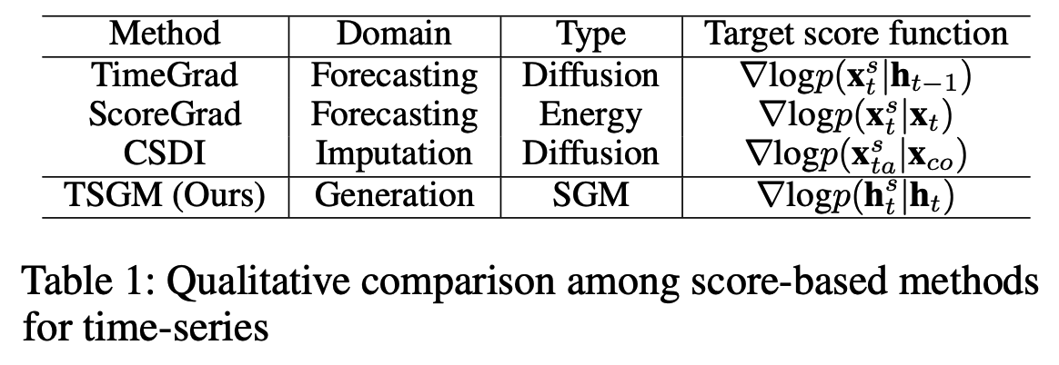
[SGMs on Time-series]

a) TimeGrad (Rasul et al. 2021)

• for time-series forecasting
• diffusion model ( = discrete version of SGMs )
• Loss: \(\sum_{t=t_0}^T-\log p_\theta\left(\mathbf{x}_t \mid \mathbf{x}_{1: t-1}, \mathbf{c}_{1: T}\right)\).
  • \(\mathbf{c}_{1: T}\) : the covariates of \(\mathbf{x}_{1: T}\).
  • by using an RNN encoder, \(\left(\mathbf{x}_{1: t}, \mathbf{c}_{1: T}\right)\) can be encoded into \(\mathbf{h}_t\).
• Sampling: forecasts future observations recursively

In the perspective of SGMs, TimeGrad and ScoreGrad can be regarded as methods to train the following conditional score network \(M\)

\(\sum_{t=t_0}^T \mathbb{E}_s \mathbb{E}_{\mathbf{x}_t^s} \mid \mid M_\theta\left(s, \mathbf{x}_t^s, \mathbf{h}_{t-1}\right)-\nabla_{\mathbf{x}_t^s} \log p\left(\mathbf{x}_t^s \mid \mathbf{h}_{t-1}\right) \mid \mid _2^2\).

b) ScoreGrad (Yan et al. 2021)

• for time-series forecasting

• energy-based generative method

  ( generalizes diffusion models into the energy-based field )

• Loss: \(\sum_{t=t_0}^T \mathbb{E}_s \mathbb{E}_{\mathbf{x}_t} \mathbb{E}_{\mathbf{x}_t^s \mid \mathbf{x}_t} \mid \mid M_\theta\left(s, \mathbf{x}_t^s, \mathbf{x}_{1: t-1}\right)-\nabla_{\mathbf{x}_t^s} \log p\left(\mathbf{x}_t^s \mid \mathbf{x}_t\right) \mid \mid _2^2\).

c) CSDI (Tashiro et al. 2021)

• for time-series imputation

  ( not only imputation, but also forecasting and interpolations )

• reconstructs an entire sequence at once, not recursively
• Loss: \(\mathbb{E}_s \mathbb{E}_{\mathbf{x}_{t a}^s} \mid \mid M_\theta\left(s, \mathbf{x}_{t a}^s, \mathbf{x}_{c o}\right)-\nabla \log p\left(\mathbf{x}_{t a}^s \mid \mathbf{x}_{c o}\right) \mid \mid _2^2\).
  • where \(\mathbf{x}_{c o}\) and \(\mathbf{x}_{t a}\) are conditions and imputation targets

Proposed TSGM

Above methods are not suitable for our generative task

• due to the fundamental mismatch between their score function definitions and generation task (Table 1)

Propose to optimize a conditional score network, by using the following denoising score matching:

• \(\mathbb{E}_s \mathbb{E}_{\mathbf{h}_{1: T}} \sum_{t=1}^T \mid \mid M_\theta\left(s, \mathbf{h}_t^s, \mathbf{h}_{t-1}\right)-\nabla_{\mathbf{h}_t^s} \log p\left(\mathbf{h}_t^s \mid \mathbf{h}_t\right) \mid \mid _2^2\).

3. Proposed Methods: TSGM

Consists of three networks:

• (1) Encoder
• (2) Decode
• (3) Conditional score network

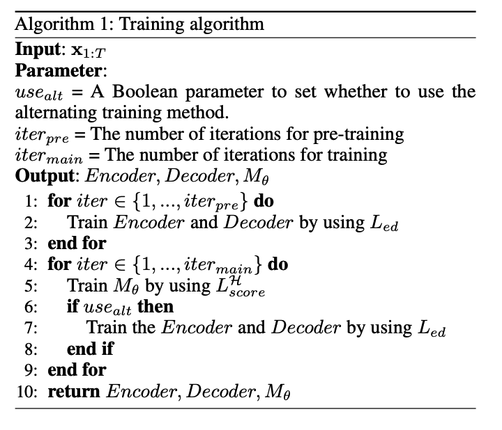
Procedures

• Step 1) Pre-train the encoder and the decoder

• Step 2) Using the pre-trained encoder and decoder, we train the conditional score network

  • will be used for sampling fake time-series.

(1) Encoder and Decoder

Notation

• \(\mathcal{X}\) and \(\mathcal{H}\) denote a data space and a latent space
• \(e\) and \(d\) are an embedding function mapping \(\mathcal{X}\) to \(\mathcal{H}\) and vice versa (= RNN)
  • \(\mathbf{h}_t=e\left(\mathbf{h}_{t-1}, \mathbf{x}_t\right), \quad \hat{\mathbf{x}}_t=d\left(\mathbf{h}_t\right)\).
• \(\mathbf{x}_{1: T}\) : time-series sample with a length of \(T\)
  • \(\mathbf{x}_t\) : multi-dimensional observation in \(\mathbf{x}_{1: T}\) at time \(t\).
• \(\mathbf{h}_{1: T}\) and \(\mathbf{h}_t\) are embedded vectors

(2) Conditional Score Network

( Unlike other domains… )

Score network for TS generation must be designed to learn the conditional log likelihood on previous generated observations

Proposed network

• Modify U-net architecture
  • modify its 2-d CNN to 1-d
• Concatenate diffused data with condition
  • use the concatenated one and temporal feature as input to learn score function

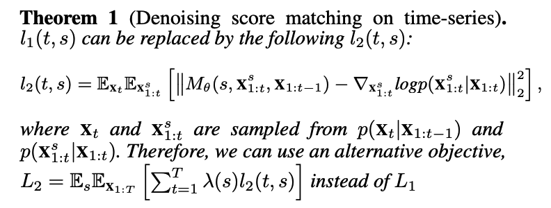
(3) Training Objective Functions

\(L_{e d}\) : train encoder & decoder

• \(L_{e d}=\mathbb{E}_{\mathbf{x}_{1: T}}\left[ \mid \mid \hat{\mathbf{x}}_{1: T}-\mathbf{x}_{1: T} \mid \mid _2^2\right]\).

\(L_{\text {score }}\) : train the conditional score network

• At time \(t\) in \([1: T]\), we diffuse \(\mathbf{x}_{1: t}\) through a sufficiently large number of steps of the forward SDE
• Notation:
  • \(\mathbf{x}_{1: t}^s\) : a diffused sample at step \(s \in[0,1]\)
  • \(M_\theta\left(s, \mathbf{x}_{1: t}^s, \mathbf{x}_{1: t-1}\right)\) : conditional score network
    • learns the gradient of the conditional log-likelihood
• \(L_1=\mathbb{E}_s \mathbb{E}_{\mathbf{x}_{1: T}}\left[\sum_{t=1}^T \lambda(s) l_1(t, s)\right]\).
  • where \(l_1(t, s)=\mathbb{E}_{\mathbf{x}_{1: t}^s}\left[ \mid \mid M_\theta\left(s, \mathbf{x}_{1: t}^s, \mathbf{x}_{1: t-1}\right)-\nabla_{\mathbf{x}_{1: t}^s} \log p\left(\mathbf{x}_{1: t}^s \mid \mathbf{x}_{1: t-1}\right) \mid \mid _2^2\right]\).
• Can use the efficient denoising score \(\operatorname{loss} L_2\) to train the conditional score network. We set \(\mathbf{x}_0=\mathbf{0}\).

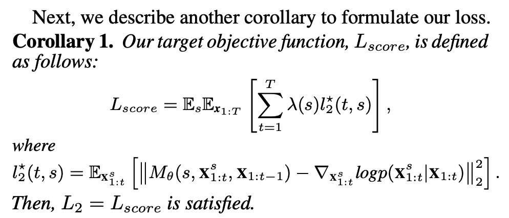
• \(L_{\text {score }}^{\mathcal{H}}=\mathbb{E}_s \mathbb{E}_{\mathbf{h}_{1: T}} \sum_{t=1}^T\left[\lambda(s) l_3(t, s)\right]\).

  with \(l_3(t, s)=\mathbb{E}_{\mathbf{h}_t^s}\left[ \mid \mid M_\theta\left(s, \mathbf{h}_t^s, \mathbf{h}_{t-1}\right)-\nabla_{\mathbf{h}_t^s} \log p\left(\mathbf{h}_t^s \mid \mathbf{h}_t\right) \mid \mid _2^2\right]\).

\(L_{\text {score }}^{\mathcal{H}}\) is what we use for our experiments (instead of \(L_{\text {score }}\)).

(4) Training & Sampling