Multi-resolution Diffusion Models for Time-Series ForecastingPermalink

ContentsPermalink

1. Abstract
2. Introduction
3. Related Works
4. Background
5. mr-Diff: Multi-Resolution Diffusion model
   1. Extracting Fine-to-Coarse Trends
   2. Temporal Multi-resolution Reconstruction
6. Experiments

0. AbstractPermalink

Diffusion model for TS

• Do not utilize the unique properties of TS data

  • TS data = Different patterns are usually exhibited at multiple scales

  $\rightarrow$ Leverage this multi-resolution temporal structure

mr-DiffPermalink

• Multi-resolution diffusion model

• Seasonal-trend decomposition

• Sequentially extract fine-to-coarse trends from the TS for forward diffusion
  • Coarsest trend is generated first.
  • Finer details are progressively added
    • using the predicted coarser trends as condition
• Non-autoregressive manner.

1. IntroductionPermalink

Multi-resolution diffusion (mr-Diff)

• Decomposes the denoising objective into several sub-objectives

ContributionPermalink

• Propose the multi-resolution diffusion (mr-Diff) model
  • First to integrate the seasonal-trend decomposition-based multi-resolution analysis into TS diffusion
• Progressive denoising in an easy-to-hard manner
  • Generate coarser signals first $\rightarrow$ then finer details.

2. Related WorksPermalink

TimeGrad (Rasul et al., 2021)Permalink

• Conditional diffusion model which predicts in an autoregressive manner
• Condition = hidden state of a RNN
• Suffers from slow inference on long TS ($\because$ Autoregressive decoding )

CSDI (Tashiro et al., 2021)Permalink

• Non-autoregressive generation
• SSL to guide the denoising process
• Needs two transformers to capture dependencies in the channel and time dimensions

• Complexity is quadratic in the number of variables and length of TS

• Masking-based conditioning
  • cause disharmony at the boundaries between the masked and observed regions

SSSD (Alcaraz & Strodthoff, 2022)Permalink

• Reduces the computational complexity of CSDI by replacing the transformers with a SSSM
• Same masking-based conditioning as in CSDI
  • still suffers from the problem of boundary disharmony

TimeDiff (Shen & Kwok, 2023)Permalink

• Non-autoregressive diffusion model
• Future mixup and autoregressive initialization for conditioning

$\rightarrow$ All these TS diffusion models do not leverage the multi-resolution temporal structures and denoise directly from random vectors as in standard diffusion models.

Multi-resolution analysis techniquesPermalink

• Besides using seasonal-trend decomposition have also been used for TS modeling
• Yu et al. (2021)
  • propose a U-Net (Ronneberger et al., 2015) for graph-structured TS
  • leverage temporal information from different resolutions by pooling and unpooling
• Mu2ReST (Niu et al., 2022)
  • works on spatio-temporal data
  • recursively outputs predictions from coarser to finer resolutions
• Yformer (Madhusudhanan et al., 2021)
  • captures temporal dependencies by combining downscaling/upsampling with sparse attention.
• PSA-GAN (Jeha et al., 2022)
  • trains a growing U-Net
  • captures multi-resolution patterns by progressively adding trainable modules at different levels.

$\rightarrow$ However, all these methods need to design very specific U-Net structures

3. BackgroundPermalink

(1) DDPMPermalink

pass

(2) Conditional Diffusion Modles for TSPermalink

pass

4. mr-Diff: Multi-Resolution Diffusion ModelPermalink

Use of multi-resolution temporal patterns in the diffusion model has yet to be explored

$\rightarrow$ Address this gap by proposing the multi-resolution diffusion (mr-Diff)

Can be viewed as a cascaded diffusion model (Ho et al., 2022)

• Proceeds in $S$ stages, with the resolution getting coarser as the stage proceeds

  $\rightarrow$ Allows capturing the temporal dynamics at multiple temporal resolutions

• In each stage, the diffusion process is interleaved with seasonal-trend decomposition

NotationPermalink

• $\mathbf{X}=\mathbf{x}_{-L+1: 0}$ and $\mathbf{Y}=\mathbf{x}_{1: H}$
• Trend component of the lookback/forecast) segment at stage $s+1$ be $\mathbf{X}_s$ / $\mathbf{Y}_s$
  • Trend gets coarser as $s$ increases
• $\mathbf{X}_0=\mathbf{X}$ and $\mathbf{Y}_0=\mathbf{Y}$.

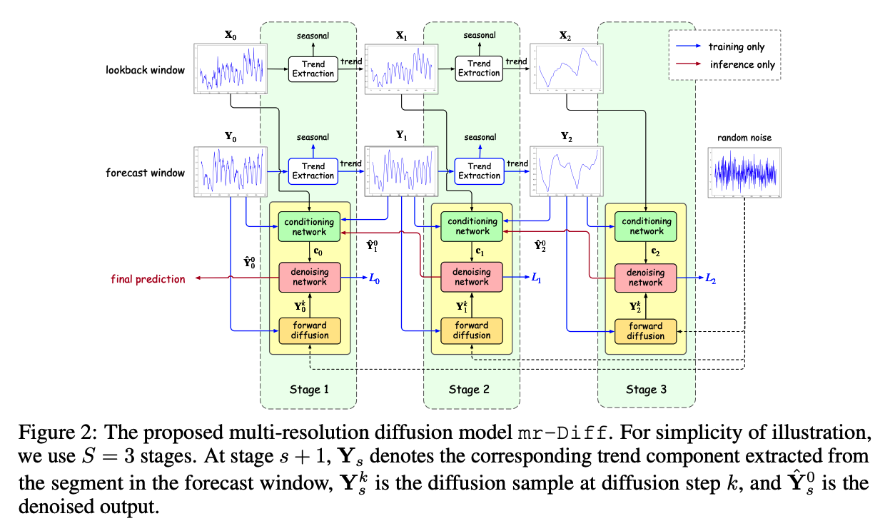
In each stage $s+1$ …

a conditional diffusion model is learned to reconstruct the “trend $\mathbf{Y}_s$ extracted from the forecast window”

Reconstruction at stage 1 then corresponds to the target TS forecast.

[ Training & Inference ]Permalink

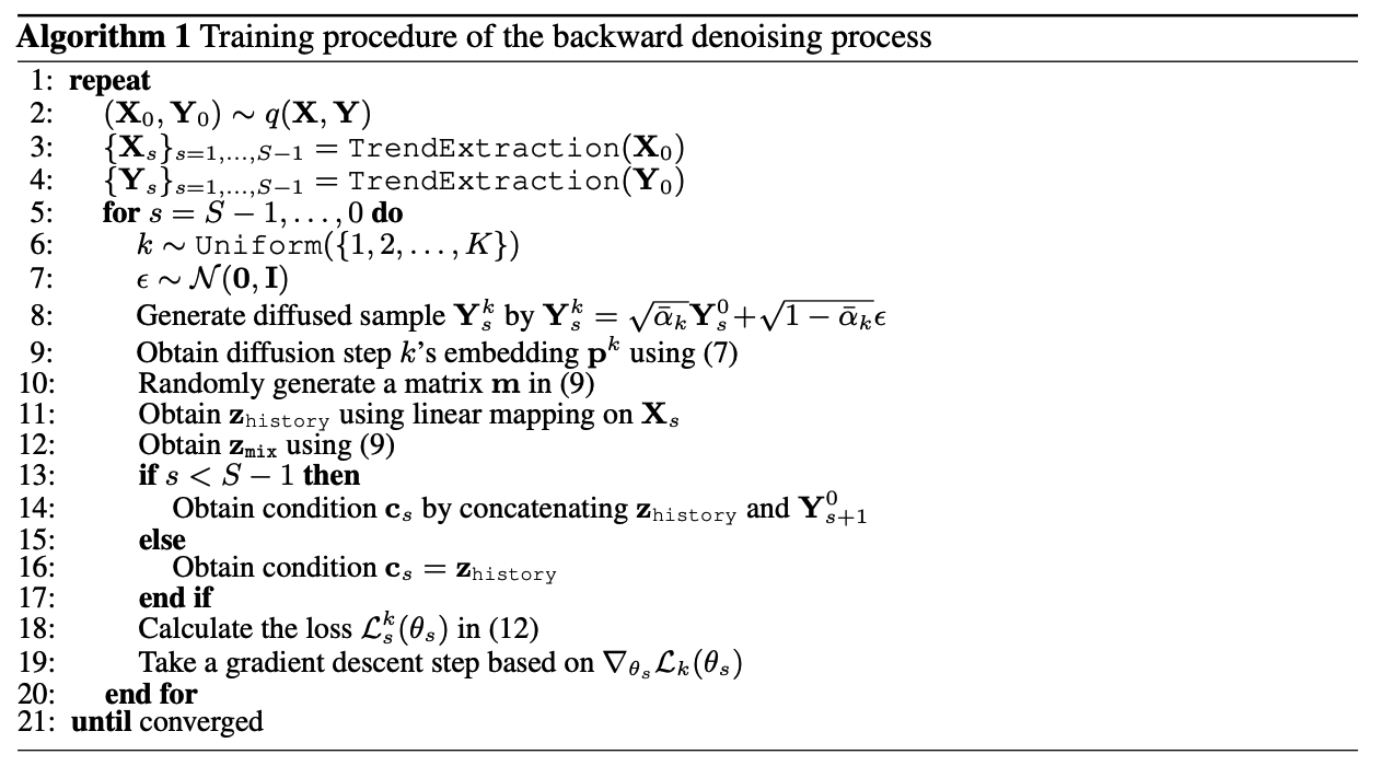
Training

• Guide the reconstruction of $\mathbf{Y}_s$
• Condition:
  • Lookback segment $\mathbf{X}_s$
  • Coarser trend $\mathbf{Y}_{s+1}$

Inference

• Ground-truth $\mathbf{Y}_{s+1}$ is not available
• Replaced by its estimate $\hat{\mathbf{Y}}_{s+1}^0$ produced by the denoising process at stage $s+1$.

(1) Extracting Fine-to-Coarse TrendsPermalink

TrendExtraction module

• $\left.\mathbf{X}_s=\text { AvgPool(Padding }\left(\mathbf{X}_{s-1}\right), \tau_s\right), s=1, \ldots, S-1$.

Seasonal-trend decomposition

• Obtains both the seasonal and trend components
• This paper focuses on trend
  • Easier to predict a finer trend from a coarser trend
  • Finer seasonal component from a coarser seasonal component may be difficult

(2) Temporal Multi-resolution ReconstructionPermalink

Sinusoidal position embeddingPermalink

$k_{\text {embedding }}=$ $\left[\sin \left(10^{\frac{0 \times 4}{w-1}} t\right), \ldots, \sin \left(10^{\frac{w \times 4}{w-1}} t\right), \cos \left(10^{\frac{0 \times 4}{w-1}} t\right), \ldots, \cos \left(10^{\frac{w \times 4}{w-1}} t\right)\right]$

• where $w=\frac{d^{\prime}}{2}$,

Passing it through….

• $\mathbf{p}^k=\operatorname{SiLU}\left(\mathrm{FC}\left(\operatorname{SiLU}\left(\mathrm{FC}\left(k_{\text {embedding }}\right)\right)\right)\right)$.

a) Forward DiffusionPermalink

$\mathbf{Y}_s^k=\sqrt{\bar{\alpha}_k} \mathbf{Y}_s^0+\sqrt{1-\bar{\alpha}_k} \epsilon, \quad k=1, \ldots, K$.

b) Backward DenoisingPermalink

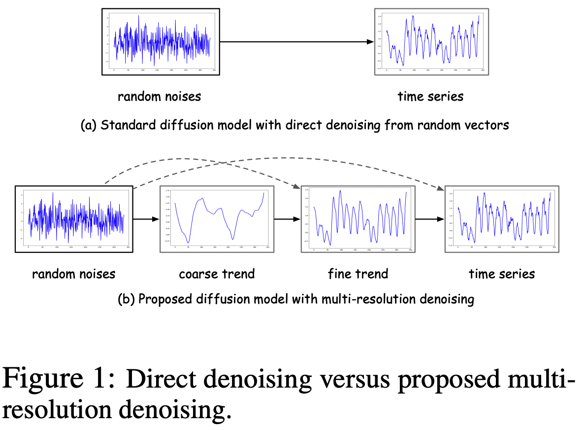
Standard diffusion models

• One-stage denoising directly

mr-Diff

• Decompose the denoising objective into $S$ sub-objectives

  $\rightarrow$ Encourages the denoising process to proceed in an easy-to-hard manner

  ( Coarser trends first, Finer details are then progressively added )

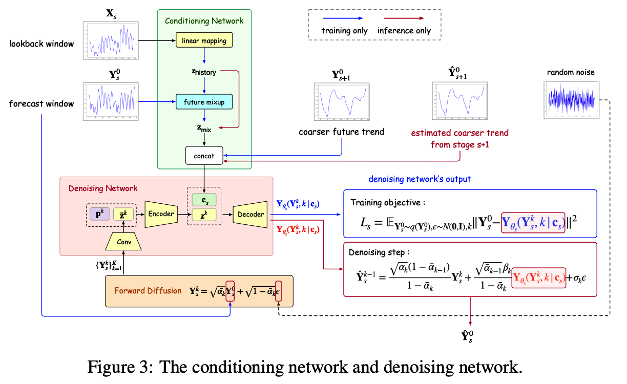
[ Conditioning network ]Permalink

Constructs a condition to guide the denoising network

Existing works

• Use the original TS lookback segment $\mathbf{X}_0$ as condition $\mathbf{c}$

mr-Diff

• Use the lookback segment $\mathbf{X}_s$ at the same decomposition stage $s$.

  $\rightarrow$ Allows better and easier reconstruction

  ( $\because$ $\mathbf{X}_s$ has the same resolution as $\mathbf{Y}_s$ to be reconstructed )

  $\leftrightarrow$ When $\mathbf{X}_0$ is used as in existing TS diffusion models, the denoising network may overfit temporal details at the finer level.

Procedures

• Step 1) Linear mapping is applied on $\mathbf{X}_s$ to produce a $\mathbf{z}_{\text {history }} \in \mathbb{R}^{d \times H}$.

• Step 2) Future-mixup: to enhance $\mathbf{z}_{\text {history }}$.

  • $\mathbf{z}_{\text {mix }}=\mathbf{m} \odot \mathbf{z}_{\text {history }}+(1-\mathbf{m}) \odot \mathbf{Y}_s^0$.

  • Similar to teacher forcing, which mixes the ground truth with previous prediction output

• Step 3) Coarser trend $\mathbf{Y}_{s+1}\left(=\mathbf{Y}_{s+1}^0\right)$ can also be useful for conditioning

  $\rightarrow$ $\mathbf{z}_{\operatorname{mix}}$ is concatenated with $\mathbf{Y}_{s+1}^0$ to produce the condition $\mathbf{c}_s$ (a $2 d \times H$ tensor).

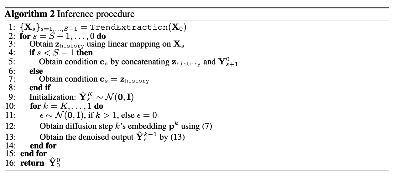
Inference

• Ground-truth $\mathbf{Y}_s^0$ is no longer available

  $\rightarrow$ No future-mixup … simply set $\mathbf{z}_{\text {mix }}=\mathbf{z}_{\text {history }}$.

• Coarser trend $\mathbf{Y}_{s+1}$ is also not available

  $\rightarrow$ Concatenate $\mathbf{z}_{\text {mix }}$ with the estimate $\hat{\mathbf{Y}}_{s+1}^0$ generated from stage $s+2$ .

[ Denoising Network ]Permalink

Outputs a $\mathbf{Y}_{\theta_s}\left(\mathbf{Y}_s^k, k \mid \mathbf{c}_s\right)$ with guidance from the condition $\mathbf{c}_s$

Denoising process at step $k$ of stage $s+1$:

• $p_{\theta_s}\left(\mathbf{Y}_s^{k-1} \mid \mathbf{Y}_s^k, \mathbf{c}_s\right)=\mathcal{N}\left(\mathbf{Y}_s^{k-1} ; \mu_{\theta_s}\left(\mathbf{Y}_s^k, k \mid \mathbf{c}_s, \sigma_k^2 \mathbf{I}\right)\right), k=K, \ldots, 1$.

• $\mathbf{Y}_{\theta_s}\left(\mathbf{Y}_s^k, k \mid \mathbf{c}_s\right)$ is an estimate of $\mathbf{Y}_s^0$.

Procedures

• Step 1) Maps $\mathbf{Y}_s^k$ to the embedding $\overline{\mathbf{z}}^k \in \mathbb{R}^{d^{\prime} \times H}$
• Step 2) Concatenate with diffusion-step $k$ ‘s embedding $\mathbf{p}^k \in \mathbb{R}^{d^{\prime}}$
• Step 3) Feed to an encoder to obtain the $\mathbf{z}^k \in \mathbb{R}^{d^{\prime \prime} \times H}$.
• Step 4) Concatenate $\mathbf{z}^k$ and $\mathbf{c}_s$ along the variable dimension
  • Form a tensor of size $\left(2 d+d^{\prime \prime}\right) \times H$.
• Step 5) Feed to a decoder
  • Outputs $\mathbf{Y}_{\theta_s}\left(\mathbf{Y}_s^k, k \mid \mathbf{c}_s\right)$.

Loss function:

• $\min _{\theta_s} \mathcal{L}_s\left(\theta_s\right)=\min _{\theta_s} \mathbb{E}_{\mathbf{Y}_s^0 \sim q\left(\mathbf{Y}_s\right), \epsilon \sim \mathcal{N}(\mathbf{0}, \mathbf{I}), k} \mid \mid \mathbf{Y}_s^0-\mathbf{Y}_{\theta_s}\left(\mathbf{Y}_s^k, k \mid \mathbf{c}_s\right) \mid \mid ^2$.

Inference

• For each $s=S, \ldots, 1$, we start from $\hat{\mathbf{Y}}_s^K \sim \mathcal{N}(\mathbf{0}, \mathbf{I})$
• Each denoising step from $\hat{\mathbf{Y}}_s^k$ (an estimate of $\mathbf{Y}_s^k$ ) to $\hat{\mathbf{Y}}_s^{k-1}$ :
  • $\hat{\mathbf{Y}}_s^{k-1}=\frac{\sqrt{\alpha_k}\left(1-\bar{\alpha}_{k-1}\right)}{1-\bar{\alpha}_k} \hat{\mathbf{Y}}_s^k+\frac{\sqrt{\bar{\alpha}_{k-1}} \beta_k}{1-\bar{\alpha}_k} \mathbf{Y}_{\theta_s}\left(\hat{\mathbf{Y}}_s^k, k \mid \mathbf{c}_s\right)+\sigma_k \epsilon$.

PseudocodePermalink

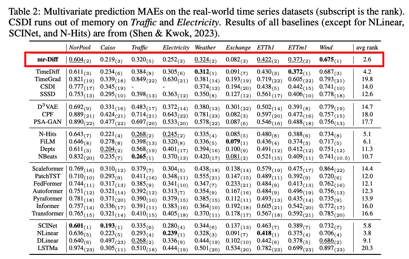
5. ExperimentsPermalink

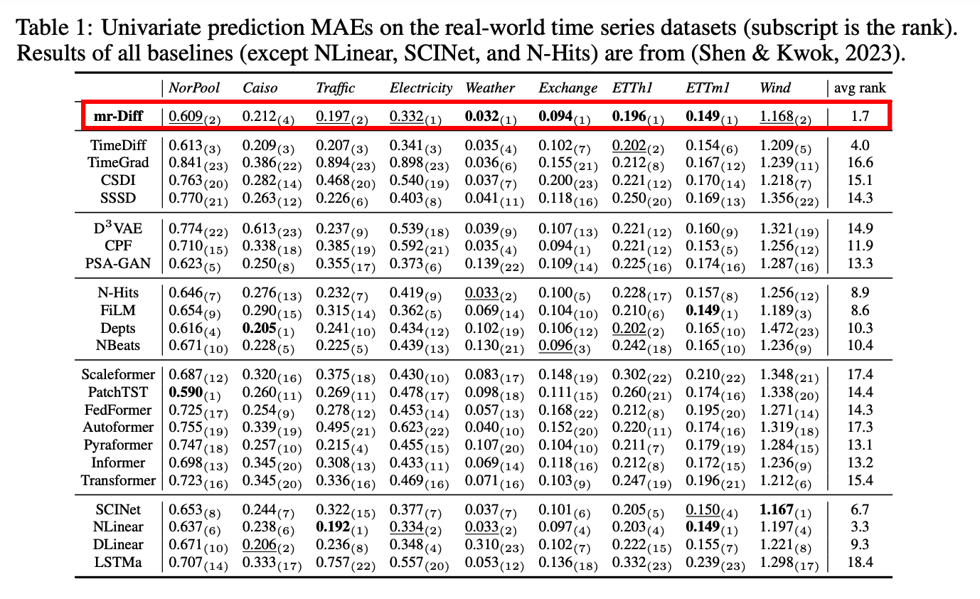
22 recent strong prediction models

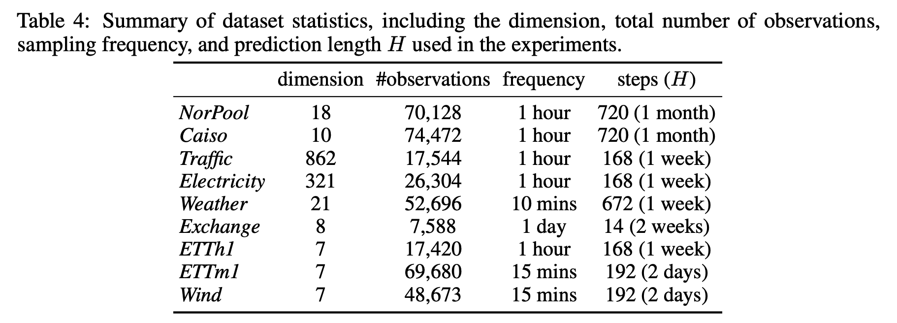
9 popular real-world time series datasets

a) Performance MeasuresPermalink

• mean absolute error (MAE)

• mean squared error (MSE)

  ( results on MSE are in Appendix K )

b) Implementation DetailsPermalink

• Adam with a learning rate of $10^{-3}$.
• Batch size is 64
• Early stopping for a maximum of 100 epochs.
• $K=100$ diffusion steps are used
  • with a linear variance schedule (Rasul et al., 2021) starting from $\beta_1=10^{-4}$ to $\beta_K=10^{-1}$
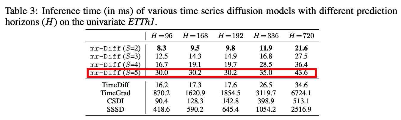
• $S=5$ stages
• History length (in $\{96,192,336,720,1440\}$ )
  • is selected by using the validation set

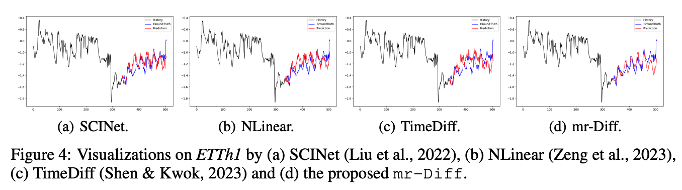
(1) Main ResultsPermalink

(2) Inference EfficiencyPermalink