(paper) GNN-based Anomaly Detection in MTS

GNN-based Anomaly Detection in MTS (2021, 32)

Contents

1. Abstract
2. Introduction
3. Proposed Framework
   1. Sensor Embedding
   2. Graph Structure Learning
   3. Graph Attention-based Forecasting
   4. Graph Deviation Scoring

0. Abstract

proposes GDN (Graph Deviation Network)

• combines a “structure learning approach” with GNN
• use attention weights to provide explainability

1. Introduction

GDP (Graph Deviation Network)

• 1) learns a graph of relationships between sensors
• 2) detects deviations from these patterns

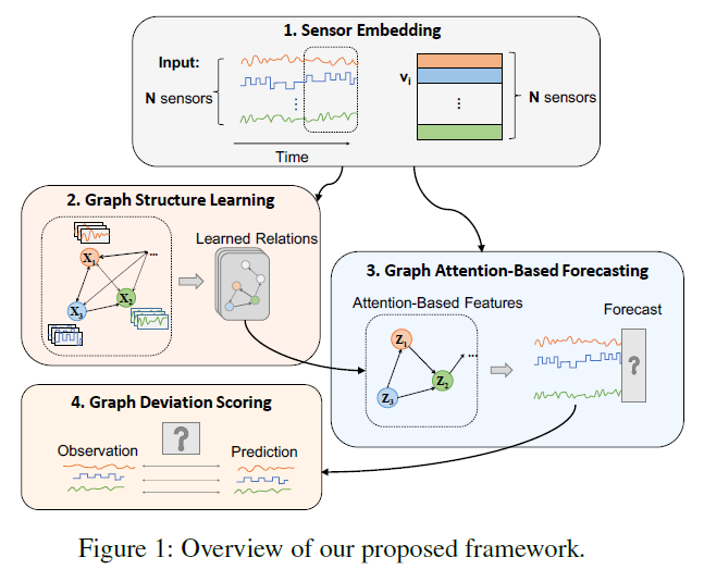
4 components

• 1) Sensor Embedding
  • capture unique characteristics of each sensor
• 2) Graph Structure Learning
  • learns relationship
• 3) Graph Attention-based Forecasting
  • predict future values
• 4) Graph Deviation Scoring
  • identifies & explains deviations

2. Proposed Framework

Problem Statement

Train data :

• \(\mathrm{s}_{\text {train }}=\left[\mathrm{s}_{\text {train }}^{(1)}, \cdots, \mathrm{s}_{\text {train }}^{\left(T_{\text {train }}\right)}\right]\).

Test data :

• \(\left[\mathrm{s}_{\text {test }}^{(1)}, \cdots, \mathrm{s}_{\text {test }}^{\left(T_{\text {test }}\right)}\right]\).

Notation

• \(N\) : # of TS (sensors)
• \(\mathrm{a}(t) \in\{0,1\}\) : whether it is anomaly or not

(1) Sensor Embedding

GOAL : represent each sensor in a flexible way

Embedding vector :

• \(\mathbf{v}_{\mathbf{i}} \in \mathbb{R}^{d}, \text { for } i \in\{1,2, \cdots, N\}\).

Details

• similar embedding = high tendency to be related
• use these embeddings in..
  • 1) structure learning
    • which sensors are related to one another
  • 2) attention mechanism
    • over neighbors

(2) Graph Structure Learning

Use “DIRECTED” graph

• sensor A is used for modeling the behavior of sensor B

Can be used in both case..

• 1) case 1 : NO prior information
• 2) case 2 : SOME prior information

about edges

Prior information

• represented as a set of “candidate relations \(\mathcal{C}_i\) “ for each sensor

  • \(\mathcal{C}_{i} \subseteq\{1,2, \cdots, N\} \backslash\{i\}\).

• compute the similarity between node \(i\)’s embedding vetor

  & embeddings of its candidates \(j \in \mathcal{C_i}\)

  • \(e_{j i} =\frac{\mathbf{v}_{\mathbf{i}}^{\top} \mathbf{v}_{\mathbf{j}}}{ \mid \mid \mathbf{v}_{\mathbf{i}} \mid \mid \cdot \mid \mid \mathbf{v}_{\mathbf{j}} \mid \mid } \text { for } j \in \mathcal{C}_{i}\).
  • \(A_{j i} =\mathbb{1}\left\{j \in \operatorname{Top} \mathrm{K}\left(\left\{e_{k i}: k \in \mathcal{C}_{i}\right\}\right)\right\}\).
    • \(k\) denotes sparsity level

With “learned adjacency matrix”, send it to graph attention-based model

(3) Graph Attention-based Forecasting

use “forecasting-based” approach

Notation

• input ( at time \(t\) ) = \(\mathbf{x}^{(t)} \in \mathbb{R}^{N \times w}\)
  • \(w\) : window size
  • \(\mathrm{x}^{(t)}:=\left[\mathrm{s}^{(\mathrm{t}-\mathrm{w})}, \mathrm{s}^{(\mathrm{t}-\mathrm{w}+1)}, \cdots, \mathrm{s}^{(\mathrm{t}-1)}\right]\).
• predict \(\mathrm{s}^{(\mathrm{t})}\)

a) Feature Extractor

• GAT based feature extractor
• incorporates the sensor embedding vectors \(\mathbf{v}_{i}\)
• node \(i\)’s aggregated representation : \(\mathbf{z}_{i}^{(t)}\).
  • \(\mathbf{z}_{i}^{(t)}=\operatorname{ReLU}\left(\alpha_{i, i} \mathbf{W} \mathbf{x}_{i}^{(t)}+\sum_{j \in \mathcal{N}(i)} \alpha_{i, j} \mathbf{W} \mathbf{x}_{j}^{(t)}\right)\).
    • \(\mathcal{N}(i)=\left\{j \mid A_{j i}>0\right\}\) : set of neighbors
    • \(\mathbf{g}_{i}^{(t)}=\mathbf{v}_{i} \oplus \mathbf{W} \mathbf{x}_{i}^{(t)}\).
    • \(\pi(i, j) =\text { LeakyReLU }\left(\mathbf{a}^{\top}\left(\mathbf{g}_{i}^{(t)} \oplus \mathbf{g}_{j}^{(t)}\right)\right)\).
    • \(\alpha_{i, j} =\frac{\exp (\pi(i, j))}{\sum_{k \in \mathcal{N}(i) \cup\{i\}} \exp (\pi(i, k))}\).
• representation of all nodes :
  • \(\left\{\mathbf{z}_{1}^{(t)}, \cdots, \mathbf{z}_{N}^{(t)}\right\}\).

b) Output Layer

Predict vector of sensor values (at time \(t\)) : \(\mathrm{s}^{(\mathrm{t})}\)

• \(\hat{\mathbf{s}}^{(\mathbf{t})}=f_{\theta}\left(\left[\mathbf{v}_{1} \circ \mathbf{z}_{1}^{(t)}, \cdots, \mathbf{v}_{N} \circ \mathbf{z}_{N}^{(t)}\right]\right)\).

Loss Function :

• \(L_{\mathrm{MSE}}=\frac{1}{T_{\text {train }}-w} \sum_{t=w+1}^{T_{\text {train }}} \mid \mid \hat{\mathbf{s}}^{(\mathrm{t})}-\mathrm{s}^{(\mathrm{t})} \mid \mid _{2}^{2}\).

(4) Graph Deviation Scoring

• detect & explain anomalies
• anomalousness score :
  • \(\operatorname{Err}_{i}(t)= \mid \mathbf{s}_{\mathbf{i}}^{(\mathbf{t})}-\hat{\mathbf{s}}_{\mathbf{i}}^{(\mathbf{t})} \mid\).
• robust normalization
  • \(a_{i}(t)=\frac{\operatorname{Err}_{i}(t)-\widetilde{\mu}_{i}}{\widetilde{\sigma}_{i}}\).
    • \(\widetilde{\mu}_{i}\) : median
    • \({\widetilde{\sigma}_{i}}\) : inter-quartile range
• overall anomalousness ( at time \(t\) )
  • \(A(t)=\max _{i} a_{i}(t)\).
• simple moving average (SMA) to generate the “smoothed scores \(A_s(t)\)”