Accurate Demand Forecasting for Retails with Deep Neural NetworksPermalink

ContentsPermalink

1. Abstract
2. Introduction
3. Problem Formulation
4. Framework
   1. Graph Attention Component
   2. Recurrent Component
   3. Variable-wise Temporal attention
   4. Autoregressive Component
   5. Final Prediction

0. AbstractPermalink

Previous Works

• prediction of each individual product item
• adopt MTS forecasting approach

$\rightarrow$ none of them leveraged “structural information of product items”

• ex) product brand / multi-level categories

Proposal : DL-based prediction model to find…

• 1) **inherent inter-dependencies **
• 2) temporal characteristics

among product items!

1. IntroductionPermalink

Univariate TS model

• ex) ARIMA, AR, MA, ARMA,…
• treat each product separately

Multivariate TS model

• take into account the “INTER-dependencies” among items
• ex) VAR

DL-based models

• ex) RNN, LSTM, GRU
• ex2) LSTNet
  • 1) CNN + GRU for MTS forecasting
  • 2) special recurrent-skip component
    • to capture very long-term periodic patterns
  • 3) assumption : all variables in MTS have same periodicity

Existing prediction methods ignore that product items have inherent structural information, e.g., the relations between product items and brands, and the relations among various product items (which may share the same multi-level categories).

Product treePermalink

• Internal nodes : product categories

• Leaf nodes : product items

• extend the product tree by incorporating product brands

  $\rightarrow$ construct a product graph structure

Product Graph structurePermalink

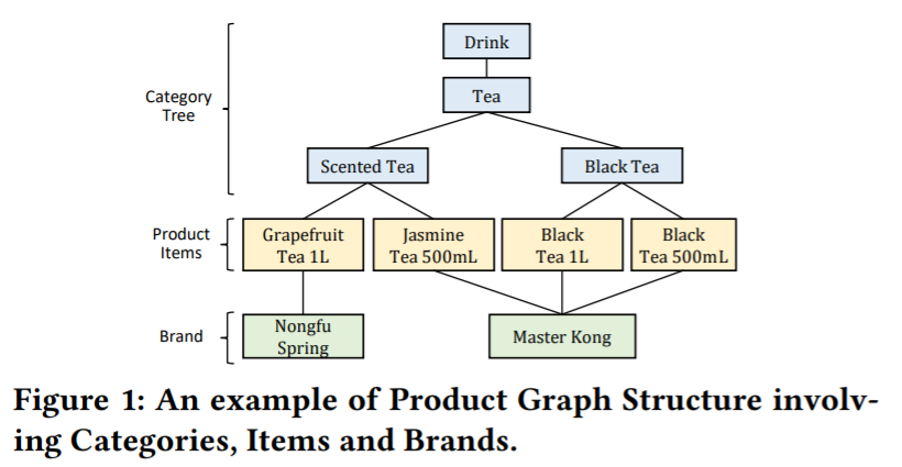
• of 4 product items

• without the product graph structure as prior…

  • case 1) treat all product items equally

  • case 2) have to implicitly infer the inherent relationship

    ( but at the cost of accuracy loss )

Structural Temporal Attention Network (STANet)Permalink

• predict product demands in MTS forecasting

• using the graph structure above

• incorporates both…

  • 1) the product graph structure ……… via GAT
  • 2) temporal characteristics of product items …… via GRU + temporal attention

• both 1) & 2) may “change over time”

  $\rightarrow$ use “attention mechanism” to deal with these

• based on “GAT”, “GRU”, “Special temporal attention”

2. Problem FormulationPermalink

Data : transaction records

• 1) time stamp
• 2) item ID
  • ( + 4 product categories & 1product brand )
• 3) amount of sold

$\rightarrow$ total of 8 fields

Pre-processing

• 1) change into MTS
• 2) for a certain category/brand : SUM

$\rightarrow$ result : MTS of volumes of product (1) items, (2) categories, (3) brands

Adjacency Matrix

• info : product graph structure

Notation

• $N_{p}$ : # of product items
• $N$ : # of product items + brands + categories
• $X=\left\{\boldsymbol{x}_{1}, \boldsymbol{x}_{2}, \ldots, \boldsymbol{x}_{T}\right\}$.
  • where $\boldsymbol{x}_{t} \in \mathbb{R}^{N \times 1}, t=1,2, \ldots, T$
• $M \in \mathbb{R}^{N \times N}$ : adjacency matrix

Goal :

• Input : $\left\{\boldsymbol{x}_{t}, \ldots, \boldsymbol{x}_{t+\tau-1}\right\}$& (fixed) $M$

• Output : $\boldsymbol{x}_{t+\tau-1+h}$
• model : $f_{M}: \mathbb{R}^{N \times \tau} \rightarrow \mathbb{R}^{N \times 1}$

Testing stage

• only need to calculate evaluation metric for the $N_{p}$

3. FrameworkPermalink

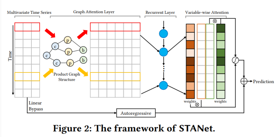
(1) Graph Attention ComponentPermalink

key point :

• capture the inter-dependencies between different variables

  $\rightarrow$ use GNN to capture it

• dynamic : “inter-dependencies may change over time!”

  $\rightarrow$ use attention mechanism

First layer : multi-head “GAT” layer

• input : $X \in \mathbb{R}^{N \times \tau}$ & $M \in \mathbb{R}^{N \times N}$

• at time step $t$….

  $\boldsymbol{h}_{t}^{i}=\sigma\left(\frac{1}{K} \sum_{k=1}^{K} \sum_{j \in \mathcal{N}_{i}} \alpha_{i j}^{k} W^{k} x_{t}^{j}\right)$.

  • $x_{t}^{j}$ : sale of variable (product, or brand, or category) $j$ at time step $t$
  • $W^{k}$ : linear transformation ( $W^{k} \in \mathbb{R}^{F \times 1}$ )

  • $\mathcal{N}_{i}$ : all the adjacent nodes of variable $i$

  • $K$ : # of multi-head attention
  • $\sigma$ : activation function
  • $\alpha_{i j}^{k}$ : coefficient

• $\alpha_{i j}^{k}=\frac{\exp \left(\operatorname{Leaky} \operatorname{ReLU}\left(f_{a}\left(W^{k} x_{t}^{i}, W^{k} x_{t}^{j}\right)\right)\right)}{\sum_{\ell \in \mathcal{N}_{i}} \exp \left(\operatorname{LeakyReLU}\left(f_{a}\left(W^{k} x_{t}^{i}, W^{k} x_{t}^{\ell}\right)\right)\right)}$.

  • $f_{a}$ : scoring function

• output : $X_{G} \in \mathbb{R}^{F N \times \tau}$

(2) Recurrent ComponentPermalink

• in the previous step…
  • variable-to-variable relationships have been processed
• use GRU as recurrent layer
• input : $X_{G} \in \mathbb{R}^{F N \times \tau}$
• notation
  • $d_r$ : hidden size of GRU
• output : $X_{R} \in \mathbb{R}^{d_{r} \times \tau}$

(3) Variable-wise Temporal attentionPermalink

previous step

• 1) GAT : captured “inter-dependencies”

• 2) recurrent component : captured “temporal patterns”

  • but, it could be “DYNAMIC”

    $\rightarrow$ use “TEMPORAL attention”

Temporal attention

• $\boldsymbol{\alpha}_{t+\tau-1}=f_{a}\left(H_{t+\tau-1}, \boldsymbol{h}_{t+\tau-1}\right)$.
  • $\boldsymbol{\alpha}_{t+\tau-1} \in \mathbb{R}^{\tau \times 1}$,
  • $f_a$ : scoring function
  • $\boldsymbol{h}_{t+\tau-1}$ : last hidden state of RNN
  • $H_{t+\tau-1}=\left[\boldsymbol{h}_{t}, \ldots, \boldsymbol{h}_{t+\tau-1}\right]$.

“VARIABLE-wise” temporal attention

• various products may have rather different temporal characteristics such as periodicity!
• $\boldsymbol{\alpha}_{t+\tau-1}^{i}=f_{a}\left(H_{t+\tau-1}^{i}, \boldsymbol{h}_{t+\tau-1}^{i}\right)$.
  • $i=$ $1,2, \ldots, d_{r}$
• attention mechanism is calculated for “a particular GRU hidden variable”
• weighted context vector of $i$th hidden variable :
  • $c_{t+\tau-1}^{i}=H_{t+\tau-1}^{i} \alpha_{t+\tau-1}^{i}$.
    • $H_{t+\tau-1}^{i} \in \mathbb{R}^{1 \times \tau}$.
    • $\boldsymbol{\alpha}_{t+\tau-1}^{i} \in \mathbb{R}^{\tau \times 1}$.
• context vector of all hidden variables :
  • $\boldsymbol{c}_{t+\tau-1}$.

Calculate the final output for horizon $h$ as

• $\boldsymbol{y}_{t+\tau-1+h}=W\left[c_{t+\tau-1} ; \boldsymbol{h}_{t+\tau-1}\right]+b$.
  • $W \in \mathbb{R}^{N \times 2 d_{r}}$ and $b \in \mathbb{R}^{1 \times 1}$

(4) Autoregressive ComponentPermalink

• just like LSTNet
• add an “autoregressive component”
  • to capture the local trend of product demands
  • linear bypass that predicts future demands from input data, to address the “scale problem”
• fit all product’s historical data into single layer

(5) Final PredictionPermalink

• integrate the outputs of the..

  • 1) neural network part
  • 2) autoregressive component

  ( using an automatically learned weight )