Bi-Mamba+; Bidirectional Mamba for Time Series Forecasting

Bi-Mamba+: Bidirectional Mamba for Time Series Forecasting

Contents

1. Abstract
2. Introduction
3. Related Work
   1. TSF
   2. SSM-based models
4. Methodology
   1. Preliminaries
   2. Overview
   3. Instance Normalization
   4. Token Generalization
   5. Mamba + Block
   6. Bidirectional Mamba+ Encoder
   7. Loss Function

0. Abstract

Mamba

• (1) “SELECTIVE” capability on input data
• (2) Hardware-aware “PARALLEL” computing algorithm

\(\rightarrow\) Balance predicting a) performance and b) computational efficiency compared to Transformers.

Bi-Mamba+

• Preserve historical information in a longer range

• Add a “FORGET gate” inside Mamba

  • Selectively combine the new & historical features

• Bi-Mamba+ = Apply Mamba+ both forward and backward

• Emphasis on both intra- or inter-series dependencies

  \(\rightarrow\) Propose a “series-relation-aware (SRA) decider”

  • controls the utilization of

    • (1) channel-independent or
    • (2) channel-mixing

    tokenization strategy for specific datasets.

1. Introduction

a) Challenges of Transformers

• Quadratic complexity of the self-attention mechanism

  \(\rightarrow\) Slow training and inference speeds.

• Do not explicitly capture the inter-series dependencies

b) State-space models (SSM)

Promising architecture for sequence modeling

Mamba

• Remarkable results in sequence processing tasks
• Key point: “selective” scanning

\(\rightarrow\) Potentially suitable for the LTSF task

c) Limited utilizations of SSM in LTSF

Stem from the inherent challenges in TS analysis tasks

• (1) Long-term TS modeling.
• (2) Emphasis on intra- or inter-series dependencies.

(1) Long-term time series modeling

• Affected by data non-stationarity, noise and outliers

• Need for patching.. Why?

  • Semantic information density of TS data at time points is lower than other types of sequence data!

  • Reduces the number of sequence elements and leads to lower computational complexity

• iTransformer (2024)
  • Simple FC layer: to map the whole sequence to hidden states
  • Coarse-grained (O), fine-grained (X) evolutionary patterns inside the TS
• This paper: model the TS in a “patching” manner

(2) Emphasis on intra- or inter-series dependencies

• Complex correlations btw multiple variables

  • CI vs. CD … not well established ( differs by datasets )

• TimeMachine (Ahamed and Cheng 2024)

  • Unified structure for

    • (1) Channel Independent (CI)
    • (2) Channel Mixing (CM,CD)

    tokenization strategiess

  • Handle both

    • (1) intra-series-emphasis
    • (2) inter-series-emphasis

  • Limitation:

    • Boundary for the selection of tokenization strategies is ambiguous

  • Statistical characteristics of datasets are overlooked.

d) Mamba+

Mamba+ = Improved Mamba block

• Adding a forget gate in Mamba

  • How: selectively combine the new features & historical features

  • Result: preserve historical information in a longer range

Bidirectional Mamba+ (BiMamba+)

• Model the MTS data from both forward and backward
• Result: Enhancing the …
  • (1) Model’s robustness
  • (2) Ability to capture interactions between TS elements
• Series-Relation-Aware (SRA) decider
  • Inspired from Spearman coefficient correlation
  • Why?? To address the varying emphasis on
    • intra-series evolutionary patterns
    • and inter-series interactions
  • How?? Measures the proportion of highly correlated series pairs in the MTS data
    • to automatically choose CI or CM tokenization strategies.
• Patch-wise tokens
  • based on the (CI or CM) tokenization strategy
  • contain richer semantic information & encourage the model to learn the long-term dependencies of the TS in a finer granularity

e) Contributions

1. Bi-Mamba+ for LTSF task
   • Improved Mamba+ block &model the MTS data from both forward and backward
2. SRA decider & Patching
   • (SRA decider) Based on the Spearman correlation coefficient to automatically choose channel independent or channel-mixing tokenization strategies.
   • (Patching) To capture long-term dependencies in a finer granularity
3. Extensive experiments on 8 real-world datasets

2. Related Work

(1) TSF

a) Transformer-based models (Vaswani et al. 2017)

Self-attention mechanism

= Quadratic complexity to the length of the sequence

\(\rightarrow\) Limitation on LTSF

b) Improvment of Transformer

• Informer (Zhou et al. 2021)
  • proposes a ProbSparse mechanism which selects top-k elements of the attention weight matrix to make distillation operation on self-attention.
• Autoformer(Wu et al. 2021)
  • uses time series decomposition and proposes an AutoCorrelation mechanism inspired by the stochastic process theory.
• Pyraformer(Liu et al. 2021)
  • introduces the pyramidal attention module to summarizes features at different resolutions and model the temporal dependencies of different ranges.
• FEDformer(Zhou et al. 2022)
  • develops a frequency enhanced Transformer through frequency domain mapping.
• PatchTST(Nie et al. 2023)
  • divides each univariate sequence into patches and uses patch-wise self-attention to model temporal dependencies.
• Crossformer(Zhang and Yan 2023)
  • adopts a similar patching operation but additionally employs a Cross-Dimension attention to capture inter-series dependencies.

Patching

• helps reduce the number of sequence elements to be processed
• extract richer semantic information

\(\rightarrow\) Still … the self-attention layers are only used on the simplified sequences.

c) iTransformer (Liu et al. 2023)

• Inverts the attention layers to straightly model inter-series dependencies.

• Limitation

  • Tokenization approach = Simply passing the whole sequence through MLP

  \(\rightarrow\) Overlooks the complex evolutionary patterns inside the TS

Transformer-based models still face the challenges in computational efficiency and predicting performance

(2) SSM-based models

a) RNNs

• Process the sequence elements step by step
• Maintain a hidden state
  • updated with each input element
• Pros & Cons
  • Pros) Simple and have excellent inference speed
  • Cons) limits the training speed and leads to forgetting long-term information

b) CNNs

• convolutional kernel to emphasis local information
• Pros & Cons
  • Pros) Parallel computing and faster training speed
  • Cons) Limits the inference speed & overlook the long-term global information.

c) State Space Models (SSM)

( Inspired by the continious system )

• (Like CNN) Fast training (Trained in parallel)
• (Like RNN) Fast inference

SSM in TSF

• SSDNet (Lin et al. 2021)
  • combines the Transformer architecture with SSM
  • provide probabilistic and interpretable forecasts
• SPACETIME(Gu et al. 2021b)
  • proposes a new SSM parameterization based on the companion matrix
  • enhance the expressivity of the model and introduces a “closed-loop” variation of the companion SSM
• Mamba(Gu and Dao 2023)
  • parameterized matrices and a hardware-aware parallel computing algorithm to SSM

• S-Mamba (Wang et al. 2024)

  • explores to use Mamba to capture inter-series dependencies of MTS
  • Procedure
    • step 1) embeds each UTS like iTransformer
    • step 2) feeds the embeddings into Mamba blocks
  • Limitation: tokenization approach may overlook the complex evolutionary patterns inside the TS

• MambaMixer (Behrouz et al. 2024)

  • adjusts the Mamba block to bidirectional
  • uses two improved blocks to capture inter & intra-series dependencies
  • Limitation: gating branch is used to filter new features of both forward and backward directions, which may cause challenges for extracting new features.

• TimeMachine (Ahamed and Cheng 2024)

  • proposes a multi-scale quadruple-Mamba architecture

    • to unify the handling of CI & CM situations

  • Limitation: CM & CI strategies are chosen simply based on the length of historical observations and variable number of different datasets.

    \(\rightarrow\) Characteristics of the MTS data are not fully considered

3. Methodology

(1) Preliminaries

Notation

• \(\mathbf{X}_{\text {in }}=\) \(\left[x_1, x_2, \ldots, x_L\right] \in \mathbb{R}^{L \times M}\),
• \(\mathbf{X}_{\text {out }}=\left[x_{L+1}, x_{L+2}, \ldots, x_{L+H}\right] \in \mathbb{R}^{H \times M}\),

State Space Models

• \(h^{\prime}(t)=\mathbf{A} h(t)+\mathbf{B} x(t), \quad y(t)=\mathbf{C} h(t)\).

  • where \(\mathbf{A} \in \mathbb{R}^{N \times N}, \mathbf{B} \in \mathbb{R}^{D \times N}\) and \(\mathbf{C} \in \mathbb{R}^{N \times D}\).

• Notation

  • \(N\): state expansion factor
  • \(D\) : dimension factor

• Continuous parameters \(\mathbf{A}, \mathbf{B}\)

  \(\rightarrow\) Discretized to \(\overline{\mathbf{A}}, \overline{\mathbf{B}}\)

  • by zero-order holding & time sampling at intervals of \(\Delta\),

Discretiztion

\(\begin{aligned} & \overline{\mathbf{A}}=\exp (\Delta \mathbf{A}), \\ & \overline{\mathbf{B}}=(\Delta \mathbf{A})^{-1}(\exp (\Delta \mathbf{A})-\mathbf{I}) \cdot \Delta \mathbf{B} . \end{aligned}\).

Discretized SSM

• \(h_k=\overline{\mathbf{A}} h_{k-1}+\overline{\mathbf{B}} x_k, \quad y_k=\mathbf{C} h_k\).

• (1) Can be trained in parallel
  • in a convolutional operation way
• (2) Efficient inference
  • in a RNN manner

HIPPO Matrix (Gu et al. 2020)

• To the initialization of matrix \(\mathbf{A}\)
• Namely the structured state space model (S4) (Gu et al. 2021b)
• Improvement on the ability to model long-term dependencies

Mamba (Gu and Dao 2023)

• Parameterizes the matrices \(\mathbf{B}, \mathbf{C}\) and \(\Delta\) in a data-driven manner

• Introducing a “selection” mechanism into \(\mathrm{S} 4\) model

• Uses a novel hardware-aware parallel computing algorithm

• Linear computational complexity

  & outstanding capabilities in modeling long-term dependencies

(2) Overview

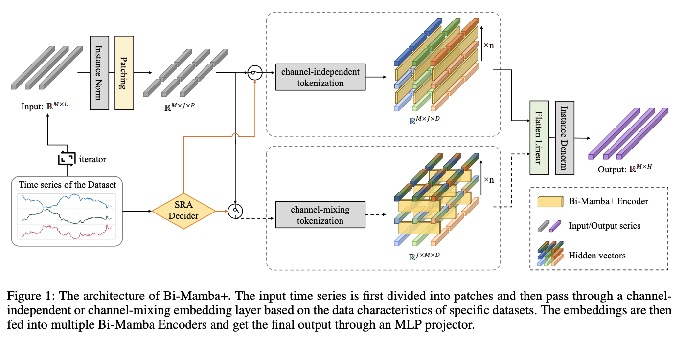
Bi-Mamba+

• Step 1) Calculate the tokenization strategy indicator
  • through the SRA decider
• Step 2) Divide the TS into patches & generate patch-wise tokens
  • based on the tokenization strategy indicator (CI or CM)
• Step 3) Fed into multiple Bi-Mamba+ encoders
• Step 4) Fatten head & linear projector

(3) Instance Normalization

Distribution shift

• Statistical properties of time series data usually change over time

RevIN (Kim et al. 2022)

• Eliminate the non-stationary statistics in the input TS

(4) Token Generalization

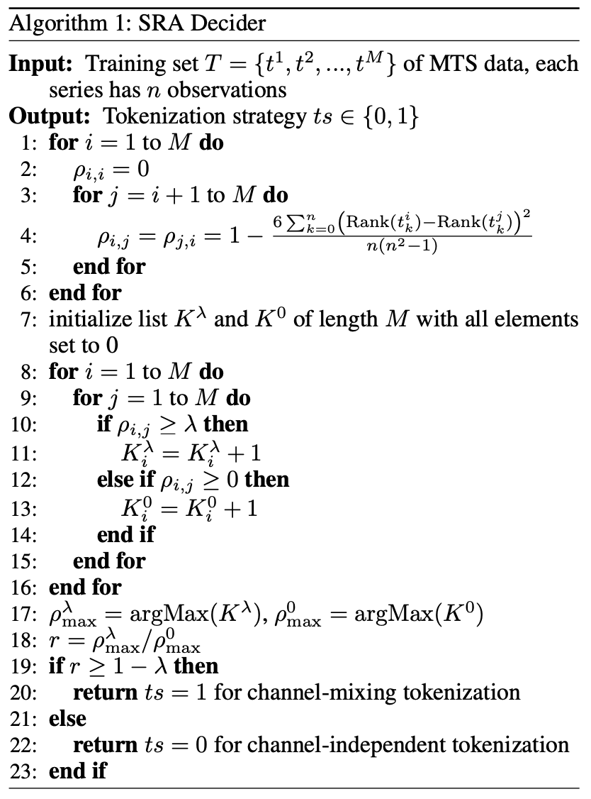
a) SRA Decider

Both CI & CD (CM) strategies can achieve SOTA accuracy

• CI wins … with datasets with few variables
• CM wins … with datasets with more variables

\(\rightarrow\) Balance between the emphasis on INTER & INTRA dependencies

SRA decider

• Automatically control the tokenization process

• Step 1) Extract the training set data \(T=\left\{t^1, t^2, \ldots, t^M\right\}\)

• Step 2) Calculate the Spearman correlation coefficients \(\rho_{i, j}\)

  • of different series \(t^i\) and \(t^j\)

  • where \(i\) and \(j\) are the indexes of the series ranging from 1 to \(M\)

• Step 3) Set threshold \(\lambda\) and 0
  • to filter out series pairs with positive correlation

• Step 4) Count the maximum number of relevant series \(\rho_{\max }^\lambda\) and \(\rho_{\max }^0\)

• Step 5) Calculate the relation ratio \(r=\rho_{\max }^\lambda / \rho_{\max }^0\).

• Step 6) Select..

  • CM strategy to generate sequence tokens for datasets with \(r \geq 1-\lambda\)
  • CI strategy otherwise

Spearman coefficient

• Nonparametric statistical indicator for evaluating the monotonic relationship between two sequences

b) Tokenization Process

Generalize patch-wise tokens to emphasize capturing local evolutionary patterns of the TS

Procedures

• Step 1) Patch UTS
  • Input: \(x_{1: L}^i\)
  • Output: \(p^i \in \mathbb{R}^{J \times P}\)
    • \(J\) : Total number of patches
    • \(P\) : Length of each patch
    • \(S\): Stride
• Step 2-1) CI strategy
  • UTS is concatenated to the tokens \(\mathbb{E}_{\text {ind }} \in \mathbb{R}^{M \times J \times D}\),
    • \(D\) : Hidden state dimension
• Step 2-2) CM strategy
  • Group patches with the same index of different series
  • Pass each group through the tokenization layer
  • Output: \(\mathbb{E}_{\text {mix }} \in\) \(\mathbb{R}^{J \times M \times D}\).

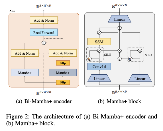
(5) Mamba+ Block

a) Mamba block

• 2 branches to process the input features, \(b_1\) & \(b_2\)
  • (branch 1) \(b_1\): Passes the input features through a 1-D CNN & SSM block
  • (branch 2) \(b_2\): Passes the input features into a SiLU activation function to serve as a gate
• HIPPO matrix (embedded in the SSM block)
  • Retain a fairly long-term historical information
  • Still …. the obtained result is filtered directly through the gate of another branch, resulting in the tendency to prioritize proximal information(Wang et al. 2024)
• Solution: improved Mamba+ block
  • specifically designed for LTSF.

b) Mamba+ block

Add a forget gate

\(\text{gate}_f=1-\text{gate}_{b_2}\),

• \(\text{gate}_f\): Forget gate
• \(\text{gate}_{b_2}\) : Result of sigmoid function in \(b_2\).

\(x^{\prime}\): Output of the 1-D CNN

• Step 1) Multiplied with gate \(_f\)
• Step 2) Added to the filtered result of SSM

\(\text{gate}_f\) & \(\text{gate}_{b_2}\) selectively combine the added new features with the forgotten historical features in a complementary manner.

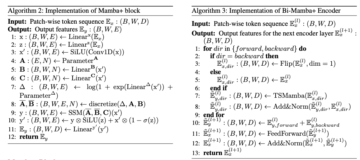
(6) Bidirectional Mamba+ Encoder

Original Mamba block

• Process 1-D sequence on one direction

Bidirectional Mamba+

• Structure to comprehensively model the MTS
• Encoder Input: \(\mathbb{E}_x^{(l)} \in \mathbb{R}^{B \times W \times D}\)
  • \(l\): encoder layer
  • \(B\) and \(W\) corresponds to \(M\) or \(J\) depending on the tokenization strategy.
  • If \(t s=1\)
    • \(\mathbb{E}_x^{(l)} \in \mathbb{R}^{J \times M \times D}\) and \(\mathbb{E}_x^{(0)}=\mathbb{E}_{m i x}\),
  • Else:
    • \(\mathbb{E}_x^{(0)}=\mathbb{E}_{m i x}\) and \(\mathbb{E}_x^{(0)}=\mathbb{E}_{\text {ind }}\).
• Two Mamba+ blocks in one Bi-Mamba+ encoder
  • to model the input sequence from the forward and backward directions respectively
  • \(\mathbb{E}_{x, d i r}^{(l)}\) where dir \(\in\{\) forward, backward \(\}\).
• \(\mathbb{E}_x^{(l+1)}=\sum_{d i r}^{\{\text {forward,backward }\}} \mathcal{F}\left(\mathbb{E}_{y, d i r}^{(l)}, \mathbb{E}_{x, d i r}^{(l)}\right)\) .
  • ( = input of the next Bi-Mamba+ encoder layer )

(7) Loss Function

MSE