MambaTS; Improved Selective SSM for LTSF

MambaTS: Improved Selective State Space Models for Long-term Time Series Forecasting

Contents

1. Abstract
2. Introduction
3. Related Work
4. Model Architecture
   1. Patching & Tokenization
   2. Variable Permutation Training (VPT)
   3. Variable-Aware Scan along Time (VAAST)
      1. Training
      2. Inference
5. Experiments

0. Abstract

Limitations of current Mamba in LTSF

MambaTS

Propose 4 targeted improvements

• (1) Variable scan along time (VST)
  • to arrange the historical information of all the variables together.
• (2) Temporal Mamba Block (TMB)
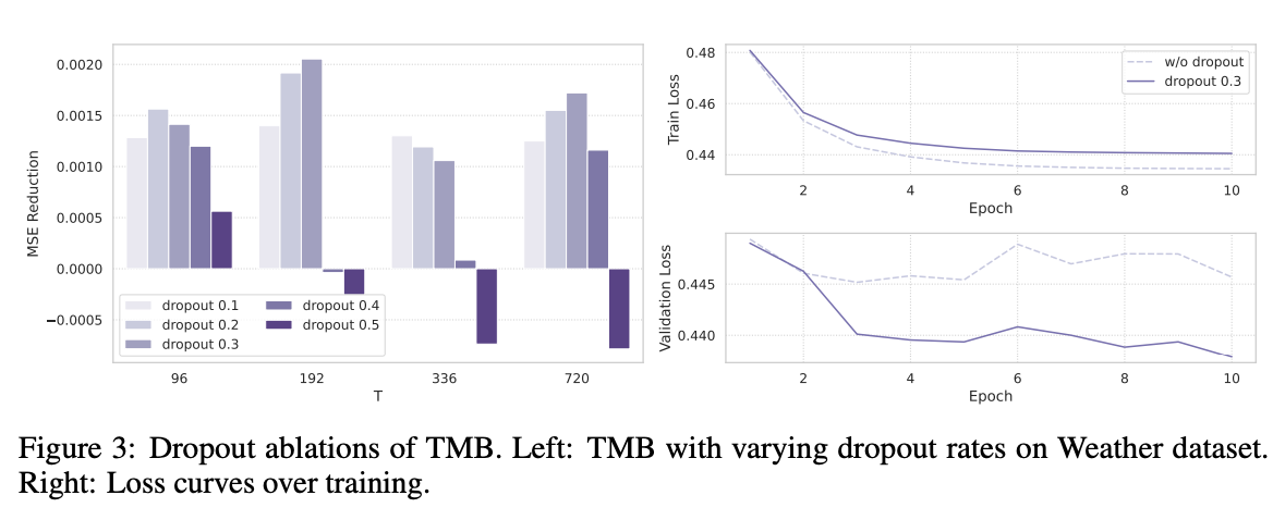
  • causal convolution (X) \(\rightarrow\) dropout (O)
• (3) Variable permutation training (VPT)
  • Tackle the issue of variable scan order sensitivity
• (4) Variable-aware scan along time (VAST)
  • dynamically discover variable relationships during training
  • decode the optimal variable scan order

1. Introduction

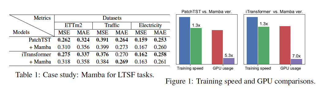
Mamba

• pros) (compared toPatchTST & Transformer)
  • x 1.3 faster
  • x 5.3 & x 7.0 memory reduction
• cons) but lacks performances

MambaTS

• (1) Variable scan along time (VST)

  • (unlike PatchTST) variable mixing manner
    • by alternately organizing the tokens of different variables at the same timestep

• (2) Temporal Mamba Block (TMB)

  • remove convolution before SSM, rather add dropout

• (3) Variable Permutation Training (VPT)

  • shffule the variable order in each iteration

    \(\rightarrow\) mitigate the impact of undefined variable roder

• (4) Variable-Aware Scan along Time (VAST)

  • Q) How to determine optimal channel order?

( Note that positional embedding is removed, following the practice of MAMBA )

2. Related Work

(1) MAMBA

To address the scan order sensitivity …

• Bidierctional scaanning [18]
• Multi-direction scanning [44,39]
• Automatic direction scanning [45]

\(\rightarrow\) Limited work considering the issue of variable scan order in temporal problems!

\(\rightarrow\) Solution: VAST strategy

3. Model Architecture

Nottion

• Input: \(\left(\mathbf{x}_1, \mathbf{x}_2, \cdots, \mathbf{x}_L\right)\), where \(\mathbf{x}_i \in \mathbb{R}^K\)
• Future: \(\left(\mathbf{x}_{L+1}, \cdots, \mathbf{x}_{L+2}, \cdots, \mathbf{x}_{L+T}\right)\)

(1) Overall Architecture

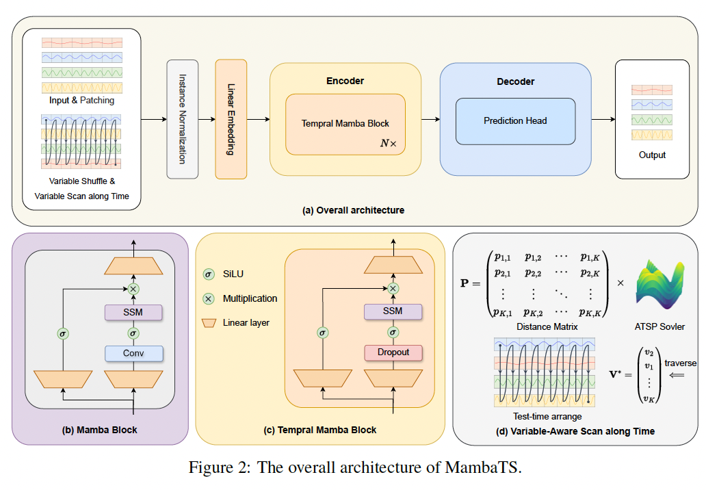
• (1) Embedding layer
• (2) Instance normalization
• (3) Temporal Mamba blocks (x N)
• (4) Prediction head

a) Patching & Tokenization

• \(M\) patches of \(D\) dimension

b) VST: Variable Scan along Time

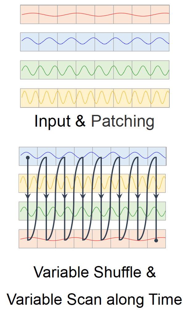
( Embed \(K\) variables \(\rightarrow\) \(K \times M\) tokens )

Arange tokens of variables at eaach time step in an alternating fashion temporally.

\(\rightarrow\) Enables the model to accuractely capture..

• (1) long-term dependencies

• (2) dynamic changes in TS data

\(\rightarrow\) Feed the results of VST into encoder

c) Encoder = TMB \(\times N\)

2 (SSM) Branches

• RIGHT: focuses on sequence modeling
• LEFT: contains a gated non-linear layer

Remove Conv, add Dropout

• (before) \(h_t=\operatorname{SSM}\left(\operatorname{Conv}\left(\operatorname{Linear}\left(\mathbf{x}_{\mathbf{t}}\right)\right)\right)+\sigma\left(\operatorname{Linear}\left(\mathbf{x}_{\mathbf{t}}\right)\right)\).
• (after) \(h_t=\operatorname{SSM}\left(\operatorname{Dropout}\left(\operatorname{Linear}\left(\mathbf{x}_{\mathbf{t}}\right)\right)\right)+\sigma\left(\operatorname{Linear}\left(\mathbf{x}_{\mathbf{t}}\right)\right)\)

d) Prediction Head

(similar to PatchTST) adopt CI decoding approach

e) Instance Normalization

Standardize each channel

(2) Variable Permutation Training (VPT)

Goal of VPT

• To mitigate the impact of undefined channel orders

  ( + augment local context interaactions)

How?

• Input: \(K \times M\) tokens.
• Shuffle them in a consistent order & revert the shuffle state after decoding

(3) Variable-Aware Scan along Time

To find the optimal scan order for inference stage

a) Training

Directed graph adjacency matrix \(\boldsymbol{P} \in \mathbb{R}^{K \times K}\)

= Cost from node \(i\) to node \(j\).

Via VPT .. explore various combinations of scan orders & evaluatae effectivness

ex) Node index sequence \(\mathbf{V}=\left\{v_1, v_2, \cdots, v_K\right\}\) i

• \(v_k\) : the new index in the shuffled sequence
• \(K-1\) transition tuples \(\left\{\left(v_1, v_2\right),\left(v_2, v_3\right), \cdots\left(v_{K-1}, v_K\right)\right\}\)
• For each sample, calculaate a training loss \(l^{(t)}\) of the \(t\)-th iteration

\(\rightarrow\) Update \(\boldsymbol{P}\) with EMA

• \(p_{v_k, v_{k+1}}^{(t)}=\beta p_{v_k, v_{k+1}}^{(t-1)}+(1-\beta) l^{(t)}\).
• \(p_{v_k, v_{k+1}}^{(t)}=\beta p_{v_k, v_{k+1}}^{(t-1)}+(1-\beta) \bar{l}(t)\)…… centralized version
  • where \(\bar{l}^{(t)}=l^{(t)}-\mu\left(l^{(t)}\right)\),

b) Inference

\(\boldsymbol{P}\) are leveraged to determine the optimal variable scan order!

This involves solving the asymmetric traveling salesman problem, which seeks the shortest path visiting all nodes.

Given the dense connectivity represented by \(\boldsymbol{P}\), finding the optimal traversal path is NP-hard.

Hence, we introduce a heuristic-based simulated annealing [47] algorithm for path decoding.

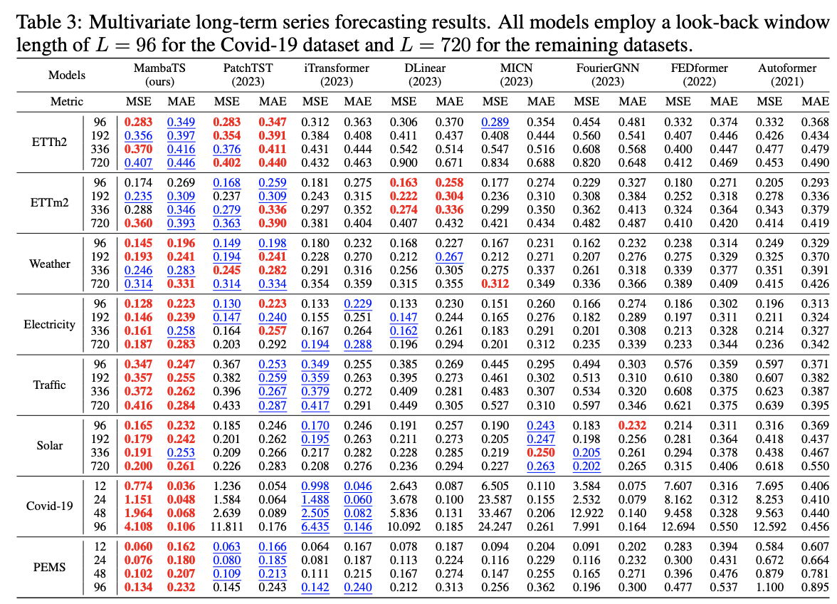
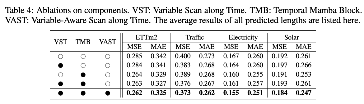
4. Experiments