Is Mamba Effective for Time Series Forecasting?

Is Mamba Effective for Time Series Forecasting?

Contents

1. Abstract

0. Abstract

Limitation of Transformer: Quadratic complexity

Solution: Mamba: Selective SSM

S-Mamba

• Simple-Mamba (S-Mamba) for TSF
• Details
  • (1) Tokenization: Tokenize the time points of each variate via a linear layer
  • (2) Encoder:
    • 2-1) “Bidirectional” Mamba layer: to extract inter-variate correlations
    • 2-2) FFN: to learn temporal dependencies
  • (3) Decoder: linear mapping layer.

https://github.com/wzhwzhwzh0921/S-D-Mamba.

1. Introduction

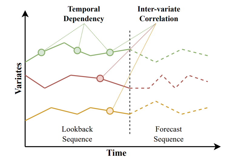
• TD: temporal dependency (intra-series)
• VC: inter-variate corrrelation (inter-series)

S-Mamba (Simple-Mamba)

• Step 1) Linear layer
  • Time points of “each variate” are tokenized
• Step 2) Mamba VC (Inter-variate Correlation) Encoding layer
  • Encodes the “VC” by utilizing a “Bidirectional” Mamba
• Step 3) FFN TD (Temporal Dependency) Encoding Layer
  • Extract the “TD” by simple FFN
• Step 4) Mapping layer
  • Output the forecast results.

Experiments

• Low requirements in GPU memory usage and training time
• Maintains superior performance compared to the SOTA models in TSF

Contributions

(1) Propose S-Mamba

• Mamba-based model for TSF

• Delegates the extraction of

  • (1) [VC] inter-variate correlations
  • (2) [TD] temporal dependencies

  to a bidirectional Mamba block and a FFN

(2) Experiments

• vs. SOTA models in TSF
• Superior forecast performance & Less computational resources

(3) Extensive experiments

2. Related Works

(1) TSF

a) Transformer-based

pass

b) Linear models

pass

(2) Application of Mamba

a) NLP

b) CV

c) Others

Tasks of predicting sequences of

• sensor data [6]
• stock prediction [50]

Sequence Reordering Mamba [60]

• Exploit the inherent valuable information embedded within the long sequences

TimeMachine

• Capture long-term dependencies in MTS

Effectively reduce the parameter size & improve the efficiency of model inference

( while achieving similar or outperforming performance )

3. Preliminaries

(1) Problem Statement

• Input: \(U_{\text {in }}=\left[u_1, u_2, \ldots, u_L\right] \in \mathbb{R}^{L \times V}\)
  • \(u_n=\left[p_1, p_2, \ldots, p_V\right]\).
• Output: \(U_{\text {out }}=\left[u_{L+1}, u_{L+2}, \ldots, u_{L+T}\right] \in\) \(\mathbb{R}^{T \times V}\).
  • \(p\) : Variate
  • \(V\) : Total number of variates

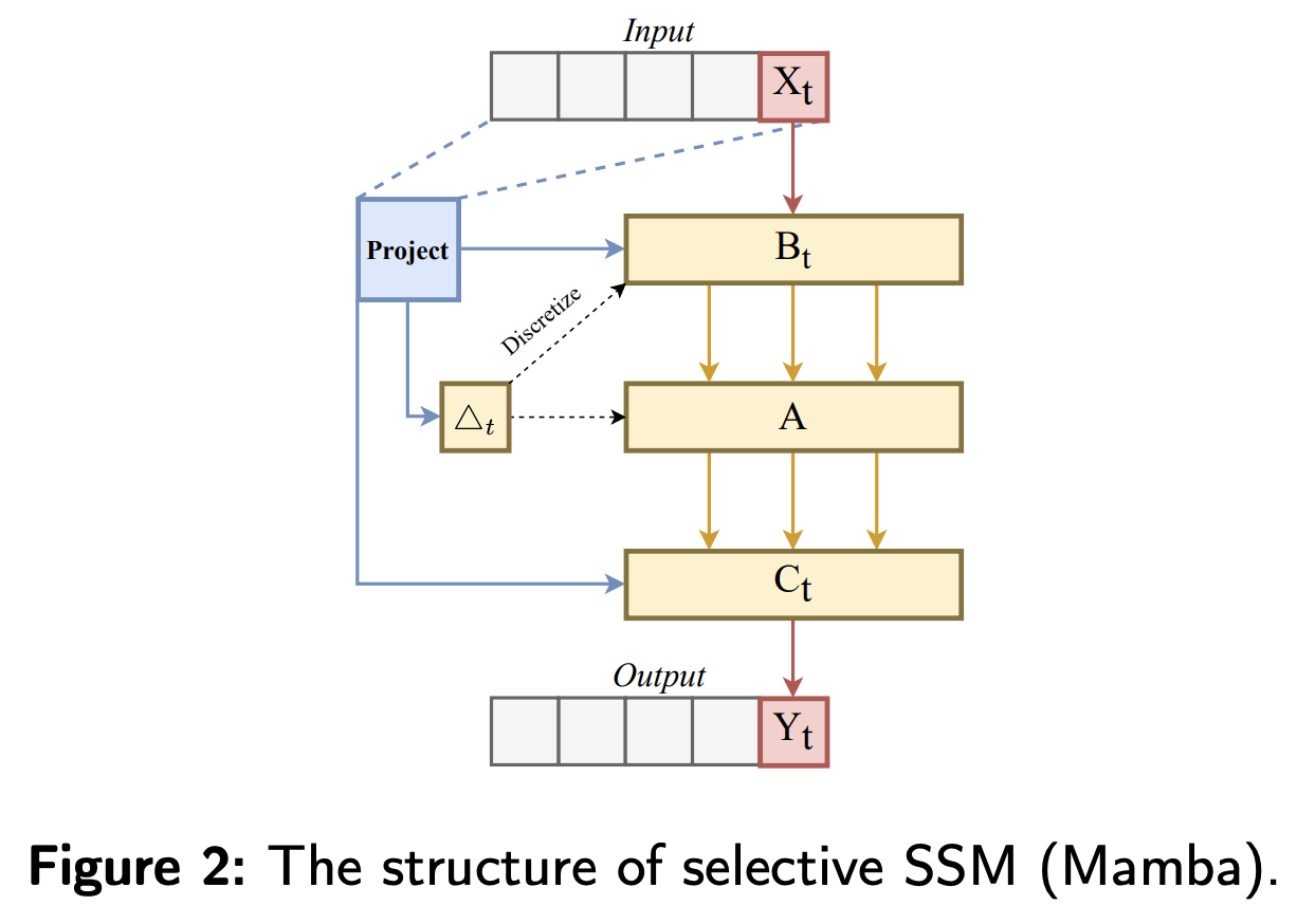
(2) SSM

Concepts

• Latent states \(h(t) \in \mathbb{R}^N\)
• Output sequences \(y(t) \in \mathbb{R}^N\)
• Input sequences \(x(t) \in \mathbb{R}^D\)

\(\begin{aligned} h(t)^{\prime} & =\boldsymbol{A} h(t)+\boldsymbol{B} x(t), \\ y(t) & =\boldsymbol{C} h(t), \end{aligned}\).

• where \(\boldsymbol{A} \in \mathbb{R}^{N \times N}\) and \(\boldsymbol{B}, \boldsymbol{C} \in \mathbb{R}^{N \times D}\) are learnable matrices

Discretiztion: discretized by a step size \(\Delta\),

Discretized SSM model

\(\begin{aligned} h_t & =\overline{\boldsymbol{A}} h_{t-1}+\overline{\boldsymbol{B}} x_t \\ y_t & =\boldsymbol{C} h_t \end{aligned}\).

• where \(\overline{\boldsymbol{A}}=\exp (\Delta A)\) and \(\overline{\boldsymbol{B}}=(\Delta \boldsymbol{A})^{-1}(\exp (\Delta \boldsymbol{A})-I) \cdot \Delta \boldsymbol{B}\).

Transitioning from

• Continuous form \((\Delta, \boldsymbol{A}, \boldsymbol{B}, \boldsymbol{C})\) to
• discrete form \((\overline{\boldsymbol{A}}, \overline{\boldsymbol{B}}, \boldsymbol{C})\),

\(\rightarrow\) Can be efficiently calculated using a linear recursive approach

Structured SSM (S4)

• Utilizes HiPPO [23] for initialization to add structure to the state matrix \(\boldsymbol{A}\),

\(\rightarrow\) Improving long-range dependency modeling.

(3) Mamba Block

Mamba

• Data-dependent “selection” mechanism into the S4
• Hardware-aware “parallel” algorithms in its looping model

\(\rightarrow\) Enables Mamba to

• capture contextual information in long sequences

• while maintaining computational efficiency.

Mamba layer takes a sequence \(\boldsymbol{X} \in \mathbb{R}^{B \times V \times D}\) as input

• \(B\) : Batch size
• \(V\) : Number of variates
• \(D\) : Hidden dimension

Mamba Block

• Step 1) Expands the $D$ to \(E D\) ( with linear projection )
  • \(E\) : block expansion factor
  • Obtain \(x\) and \(z\)
• Step 2) Conv1D + SiLU
  • Obtain \(x^{'}\)
• Step 3) Generate state representation \(y\) ( with discretized SSM )
• Step 4) \(y\) is combined with a residual connection from \(z\) after activation
  • Obtain final output \(y_t\)

\(\rightarrow\) Mamba Block effectively handles sequential information

• by leveraging selective SSM and input-dependent adaptations

4. Methodology

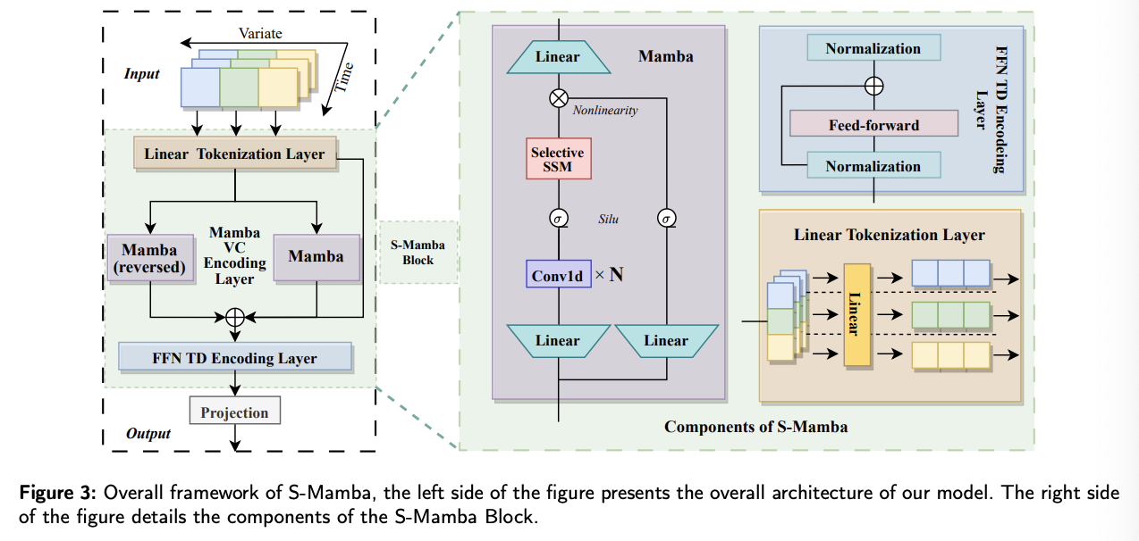
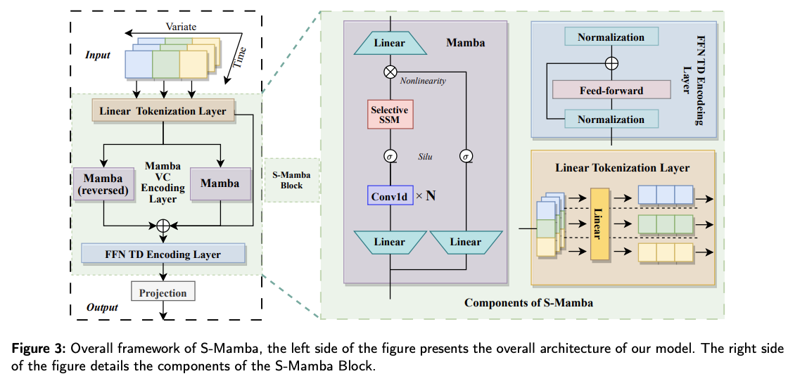
Overall structure of S-Mamba

Composed of four layers

• (1) Linear Tokenization Layer
• (2) Mamba intervariate correlation (VC) Encoding layer
  • employs a “bidirectional” Mamba block
  • capture mutual information “among variates”
• (3) FFN Temporal Dependencies (TD) Encoding Layer
  • learns the “temporal” sequence information
  • generates future series representations by a FFN
• (4) Projection Layer
  • Map the processed information of the above layers as the model’s forecast

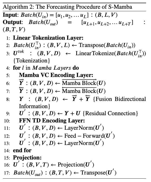
(1) Linear Tokenization Layer

\(\boldsymbol{U}=\operatorname{Linear}\left(\operatorname{Batch}\left(\boldsymbol{U}_{\text {in }}\right)\right)\).

• Input: \(U_{i n}\).

• Output: \(\boldsymbol{U}\)

(2) Mamba VC Encoding Layer

Goal: extract the VC by linking variates that exhibit analogous trends

Why not Transformer?

• Computational load of global attention escalates exponentially with an increase in the number of variates

Why Mamba?

• Mamba’s selective mechanism solves this propelm!

But Mamba….

• Transformer) undirectional

• Mamba) unidirectional

  \(\rightarrow\) Capable only of incorporating antecedent variates

  \(\rightarrow\) Employ “two” Mamba blocks to be combined as a bidirectional Mamba layer

Bidirectional Mamba: \(\boldsymbol{Y}=\overrightarrow{\boldsymbol{Y}}+\overleftarrow{\boldsymbol{Y}}\),

• \(\overrightarrow{\boldsymbol{Y}}=\overrightarrow{\operatorname{Mamba} \operatorname{Block}}(\boldsymbol{U})\).
• \(\overleftarrow{\boldsymbol{Y}}=\overleftarrow{\operatorname{Mamba\operatorname {Block}}(\boldsymbol{U})}\).

\(\rightarrow\) \(\boldsymbol{U}^{\prime}=\boldsymbol{Y}+\boldsymbol{U}\).

(3) FFN TD Encoding Layer

Step 1) Normalization layer

Step 2) FFN

• Encodes observed time series of each variate

  ( implicitly encodes TD by keeping the sequential relationships )

• Decodes future series representations using dense non-linear connections.

Step 3) Normalization layer

(4) Projection Layer

Tokenized temporal information is reconstructed