TimeMachine; A Time Series is Worth 4 Mambas for Long-term Forecasting

TimeMachine: A Time Series is Worth 4 Mambas for Long-term Forecasting

Contents

1. Abstract
2. Introduction
3. Related Works
4. Proposed Method

0. Abstract

TimeMachine

• Leverages “Mamba” to capture long-term dependencies in MTS

• Exploits the unique properties of TS data to produce salient contextual cues at “Multi-scales”

• Integrated quadruple-Mamba architecture,

  to unify the handling of

  • (1) channel-mixing and
  • (2) channel-independence situations

https://github.com/Atik-Ahamed/TimeMachine

1. Introduction

Pre-defined small patch length

• only provides contexts at a FIXED temporal or frequency resolution

\(\rightarrow\) Sensible to supply “multiscale” contexts

TimeMachine

1. Captures long-range dependencies

• by providing sensible “multi-scale” contexts and particularly enhancing local contexts in the CI situation

1. “Mamba”: Selective scan SSM

2. Exploits the unique property of TS data in a bottom-up manner

   • By producing contextual cues at “two scales”
     • via resolution reduction (or downsampling) using linear mapping
   • 1st level = high resolution
   • 2nd level = low resolution

   \(\rightarrow\) At each level, employ two Mamba modules

   • global perspectives for CM
   • global and local perspectives for the CI

Summary

1. TimeMachine
   • First to leverage purely SSM modules to capture long-term dependencies in MTS
   • Linear scalability
   • Small memory footprints superior
2. Innovative architecture
   • Unifies the handling of CM & CI situations with 4 SSM modules
   • Effectively select contents for prediction against global and local contextual information, at different scales in the MTS
3. Experiments

2. Related Works

pass

3. Proposed Method

Dataset \(\mathcal{D}\)

• Input sequence: \(x=\left[x_1, \ldots, x_L\right]\), with each \(x_t \in \mathcal{R}^M\)
• Output sequence: \(\left[x_{L+1}, \ldots, x_{L+T}\right]\).

(1) Normalization

\(x^{(0)}=\operatorname{Normalize}(x)\).

• \(x^0=\left[x_1^{(0)}, \cdots, x_L^{(0)}\right] \in \mathcal{R}^{M \times L}\),

Two options

• (1) Reversible instance normalization (RevIN)
• (2) \(Z\)-score normalization
  • \(x_{i, j}^{(0)}=\left(x_{i, j}-\operatorname{mean}\left(x_{i, j}\right)\right) / \sigma_j\),
  • where \(\sigma_j\) is the standard deviation for channel \(j\), with \(j=1, \cdots, M\).

(2) CM vs CI

Handle both CI & CM cases

Regardless of the case, TimeMachine accepts …

• input of the shape \(B M L\)
• output fo shape \(BMT\)

Channel independence (CI)

• Effective in reducing overfitting
• Helpful for datasets with a “smaller” number of channels

Channel mixing (CM)

• For datasets with a number of channels comparable to the look-back, channel mixing is more effective in capturing the correlations among channels

Shape

• CI: Input from \(B M L\) to \((B \times M) 1 L\) after the normalization
• CM: No reshaping

(3) Embedded Representations

Two-stage embedded representations

\(x^{(1)}=E_1\left(x^{(0)}\right), \quad x^{(2)}=E_2\left(D O\left(x^{(1)}\right)\right)\).

• \(D O\) : Dropout operation
• Embedding operations (via MLPs)
  • \(E_1: \mathbb{R}^{M \times L} \rightarrow \mathbb{R}^{M \times n_1}\) ,
  • \(E_2: \mathbb{R}^{M \times n_1} \rightarrow \mathbb{R}^{M \times n_2}\) .

For the CM

• \(B M n_1 \leftarrow E_1(B M L)\),
• \(B M n_2 \leftarrow E_2\left(B M n_1\right)\).

\(\rightarrow\) FIXED-length tokens of \(n_1\) and \(n_2\)

• values from the set \(\{512,256,128,64,32\}\) satisfying \(n_1>n_2\).

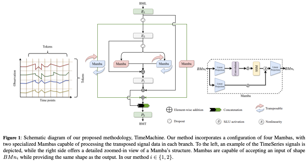
(4) Integrated Quadruple Mambas

Two processed embedded representations from \(E_1, E_2\),

Now, leverge Mamba!!

Input to one of the 4 Mamba blocks = \(u\)

• \(u\) is either \(D O\left(x^{(1)}\right)\) or \(D O\left(x^{(2)}\right)\)

  • Inner 2 mambas: \(D O\left(x^{(2)}\right)\)

  • Outer 2 mambas: \(D O\left(x^{(1)}\right)\)

• may be reshaped per CM or CI cases

Mamba block

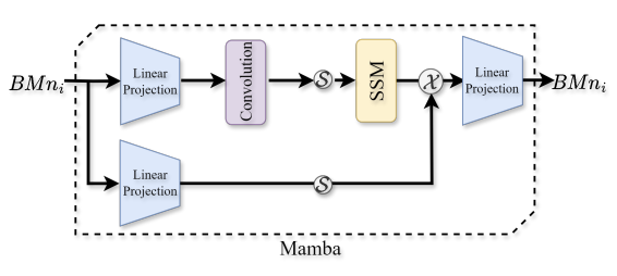
• Two FC layers in two branches
• CNN & SiLU

Continuous-time SSM

Notation

• Input function (sequence) \(u(t)\)
• Output function (sequence) \(v(t)\)
• Latent state \(h(t)\)

\(d h(t) / d t=A h(t)+B u(t), \quad v(t)=C h(t)\).

• \(h(t)\) : \(N\)-dim
  • \(N\): state expansion factor
• \(u(t)\) : \(D\)-dim
  • \(D\): dimension factor for an input token
• \(v(t)\) : \(D\)-dim

( \(A, B\), and \(C\) are coefficient matrices of proper sizes )

Discrete SSM

\(h_k=\bar{A} h_{k-1}+\bar{B} u_k, \quad v_k=C h_k\).

• where \(h_k, u_k\), and \(v_k\) are respectively samples of \(h(t), u(t)\), and \(v(t)\) at time \(k \Delta\),

\(\bar{A}=\exp (\Delta A), \quad \bar{B}=(\Delta A)^{-1}(\exp (\Delta A)-I) \Delta B\).

( For SSMs, diagonal \(A\) is often used. )

Mamba makes \(B, C\), and \(\Delta\) linear time-varying functions

( = dependent on the input )

Details

• Token \(u, B, C \leftarrow \operatorname{Linear}_N(u)\),
• \(\Delta \leftarrow\) softplus(parameter + Linear \(_D\left(\right.\) Linear \(\left.\left._1(u)\right)\right)\),
  • where \(\operatorname{Linear}_p(u)\) is a linear projection to a \(p\)-dim space
• Model dimension factor \(D\)
• Controllable dimension expansion factor \(E\).

Processed embedded representation with …

• tensor size \(B M n_1\) : transformed by outer Mambas ( input: \(D O\left(x^{(1)}\right)\) )
• tensor size \(B M n_2\) : transformed by inner Mambas ( input: \(D O\left(x^{(2)}\right)\) )

a) CM case

Whole UTS of each channel is used as a token

• with dimension factor \(n_2\) for the “inner” Mambas.

a-1) Inner Mambas

Outputs from the left-side and right-side inner Mambas:

\(x^{(3)}=v_L \bigoplus v_R \bigoplus x^{(2)}\),

• \(v_L=\left[v_{L, 1}, \cdots, v_{L, M}\right] \in \mathcal{R}^{M \times n_2}\).
• \(v_R=\left[v_{R, 1}, \cdots, v_{R, M}\right] \in \mathcal{R}^{M \times n_2}\).

Linearly mapped to \(x^{(4)}\)

• with \(P_1: x^{(3)} \rightarrow x^{(4)} \in \mathcal{R}^{M \times n_1}\).

a-2) Outer Mambas

• same … \(v_{L, k}^*, v_{R, k}^* \in \mathcal{R}^{n_1}\)
• obtain \(x^{(5)} \in \mathcal{R}^{M \times n_1}\).

b) CI case

Input is reshaped … \(B M L \mapsto(B \times M) 1 L\),

Embedded representations become \((B \times M) 1 n_1\) and \((B \times M) 1 n_2\).

b-1) One Mamba

( in each pair of outer Mambas or inner Mambas )

• considers the input dimension as 1 and the token length as \(n_1\) or \(n_2\)

b-2) Other Mamba

( in each pair of outer Mambas or inner Mambas )

• learns with input dimension \(n_2\) or \(n_1\) and token length 1

\(\rightarrow\) Enables learning both global context and local context simultaneously

Channel mixing (CM)

• Datasets with a significantly “large number of channels”

  ( when the look-back \(L\) is comparable to the channel number \(M\) )

• All 4 Mambas are used to capture the global context of the sequences at different scales and learn from the channel correlations.
• This helps stabilize the training and reduce overfitting with large M.
• To switch between the CI & CM cases, the input sequence is simply transposed, with one Mamba in each branch processing the transposed input, as demonstrated in Figure 1. These integrated Mamba blocks empower our model for contentdependent feature extraction and reasoning with long-range dependencies and feature interactions.

(5) Outer Projection

Project these tokens to generate predictions with the desired sequence length.

Two MLPs, \(P_1\) and \(P_2\), which output \(n_1\) and \(T\) time points, respectively, with each point having \(M\) channels.

Specifically, projector \(P_1\) performs a mapping \(\mathcal{R}^{M \times n_2} \rightarrow \mathcal{R}^{M \times n_1}\),

as discussed above for obtaining \(x^{(4)}\).

Subsequently, projector \(P_2\) performs a mapping \(\mathbb{R}^{M \times 2 n_1} \rightarrow \mathbb{R}^{M \times T}\), transforming the concatenated output from the Mambas into the final predictions. The use of a two-stage output projection via \(P_1\) and \(P_2\) symmetrically aligns with the two-stage embedded representation obtained through \(E_1\) and \(E_2\).

In addition to the token transformation, we also employ residual connections. One residual connection is added before \(P_1\), and another is added after \(P_1\). The effectiveness of these residual connec-