FinTSB; A Comprehensive and Practical Benchmark for Financial Time Series Forecasting

FinTSB: A Comprehensive and Practical Benchmark for Financial Time Series Forecasting

(https://arxiv.org/pdf/2502.18834)

Contents

1. Introduction
   1. FinTS forecasting
   2. Categorization of FinTS methods
   3. Lack of comprehensive benchmarks
   4. Solution: FinTSB
2. Preliminaries
   1. Problem Definition
   2. Sequence Characteristics
3. FinTSB
   1. Dataset Details
   2. Comparison Baselines
   3. Evaluation Metrics
   4. Unified Pipeline
4. Experiments
   1. Experiment Setup
   2. Trading Protocols
   3. Experimental Results
   4. Transfer Learning Results
   5. Inference Efficiency
5. Conclusion

Abstract

Financial time series (FinTS)

\(\rightarrow\) Three systemic limitations in the evaluation of the area

a) Limitations

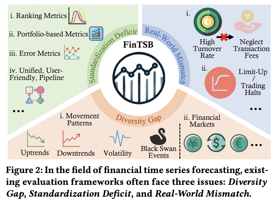
• (1) Diversity Gap
  • Failure to account for the full spectrum of stock “movement patterns”
• (2) Standardization Deficit
  • Absence of “unified” assessment protocols
• (3) Real-World Mismatch
  • Neglect of “critical market structure factors”

b) Proposal: FinTSB

Comprehensive and practical benchmark for FinTSF

• Solve (1) Diversity Gap:

  \(\rightarrow\) Categorize movement patterns into “four specific parts”

• Solve (2) Standardization Deficit:

  \(\rightarrow\) Standardize the metrics across “three dimensions”

  \(\rightarrow\) Build a user-friendly, lightweight pipeline incorporating methods from various backbones

• Solve (e) Real-World Mismatch:

  \(\rightarrow\) Extensively model “various regulatory constraints”, including transaction fees, among others.

1. Introduction

(1) Financial time series (FinTS) forecasting

a) Financial time series

Def) Sequence of data points which …

• Represent asset price factors (or market indicators)
• Reflect the dynamic behavior of financial markets

b) Financial time series (FinTS) forecasting

( Unlike general TS prediction challenges … )

Stock prices are not merely statistical series ,

but the manifestation of complex, often chaotic human behavior

( Shaped by many cognitive, emotional, and sociopolitical factors )

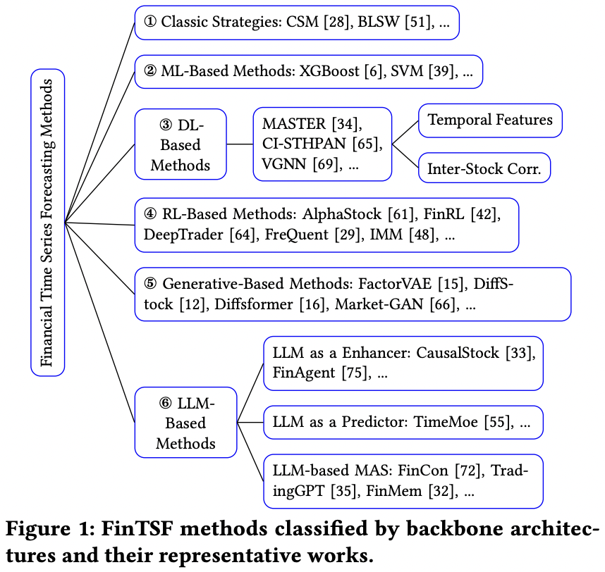
(2) Categorization of FinTSF methods

Six types based on their underlying backbone

• [Early methods] Derived from practitioner experience
  • (1) Classic strategies
    • Momentum [28] and mean reversion [51]
  • (2) ML methods
    • ARIMA [4], XGBoost [6], LightGBM [30], and Random Forests [78]
• [Recent methods] Non-linear relationships
  • (3) DL methods
    • Based on RNN, CNN, Transformer, Mamba, GNN
    • To model both stock features and inter-stock correlations
    • Dominant paradigm in the FinTSF field
  • (4) RL-based methods
    • To better optimize sequential decision making processes
    • End-to-end optimization of some key non-differentiable metrics (such as the sharpe ratio, maximum drawdown)
  • (5) Generative model-based methods
    • VAE and Diffusion Models
    • Reflect the heightened levels of uncertainty characteristic of the market, accounting for the low signal-to-noise FinTS
  • (6) LLMs
    • Process vast amounts of unstructured data and perform sophisticated reasoning
    • e.g., Enhancer [33, 75]
      • Utilize news sentiment and other textual information to augment decision making
    • e.g., Predictor [40, 55]
      • Leverage extensive TS training to generalize effectively across different domains
    • e.g., LLM-based multi-agent systems (MAS) [32, 35, 72]
      • Autonomous agents are employed to replicate decision-making processes, communication, and interactions

(3) Lack of comprehensive benchmarks

Demand for comprehensive & practical empirical evaluations!

Nonetheless… existing evaluation frameworks often face challenges!

• (1) Diversity Gap
• (2) Standardization Deficit
• (3) Real-World Mismatch

(4) Solution: FinTSB

Novel evaluation framework

\(\rightarrow\) To enhance the robustness and applicability of empirical assessments!

a) Diversity Gap

[Case 1] Different phases of stock movement

• (1) Uptrends
• (2) Downtrends
• (3) Periods of volatility
• (4) Extreme events (black swan events)

Dataset A vs. B

• Dataset (A): Contain only 3~5 years of historical data

  \(\rightarrow\) Fails to comprehensively represent all possible movement patterns

• Dataset (B): Decades of data

  \(\rightarrow\) Suffer from severe distribution shifts

[Case 2] Distinct characteristics in different markets

Dataset C vs. D

• Dataset (C) Chinese stock market
  • High retail participation & higher volatility
• Dataset (D) U.S. stock market
  • More balanced mix of institutional and retail investors & Generally higher degree of efficiency

\(\rightarrow\) Some existing works evaluate models in only one market!

Proposal: Emphasizes the diversity of FinTS

• a) Comprehensiveness of movement patterns
  • Fine-grained analysis of how different methods perform over different periods of market volatility
• b) Broad scope of financial markets

b) Standardization Deficit

Discrepancies in evaluation criteria

\(\rightarrow\) Inconsistencies in performance comparisons

Solution: Classify the current evaluation metrics into 3 main categories

• (1) Ranking metrics
  • Assess the distribution between predicted and actual daily returns
• (2) Portfolio-based metrics
  • Evaluate the profitability and risk of investment strategies derived from predictions
• (3) Error metrics
  • Quantify the degree of approximation between predicted and true values

\(\rightarrow\) Note that forecasting errors show little correlation with overall investment returns

Lack a standardized pipeline for evaluation

\(\rightarrow\) Need for a unified, user-friendly, and lightweight evaluation framework

c) Real-world Alignment

Stringent requirements for simulating realistic trading conditions

\(\rightarrow\) Recent works overlooks these constraints!

Example)

• (1) Some models still assume short selling in the Chinese A-share market

  \(\rightarrow\) Impractical due to restrictions in certain sectors

• (2) Do not take transaction fees into account

  \(\rightarrow\) Critical when constructing portfolios based on the prediction of stocks with top-𝑘 returns.

Proposal: Emphasize the necessity of incorporating these real-world constraints into evaluations

Contribution

1. Diversity Inclusion
   • Collect and pre-process tokenization historical financial TS data
   • Captures all types of movement patterns across various markets.
2. Standardization Consistency
   • Comprehensive evaluation of the capabilities of various methods from three perspectives
   • (1) Ranking & (2) Portfolio & (3) Error
3. Real-World Alignment
   • We meticulously design investment strategies that align with real-world market conditions, facilitating practical implementation in actual trading environments.
4. In-depth Evaluation
   • Evaluate a wide range of FinTSF methods
   • Extract key insights that advance the understanding of model performance in the context of financial TS forecasting

2. Preliminaries

(1) Problem Definition

a) Stock Context

\(S=\left\{s_1, s_2, \ldots, s_N\right\} \in \mathbb{R}^{N \times L \times F}\): Set of all stocks

• \(s_i\): Specific stock

  • \(s_i^t \in \mathrm{R}^F\): Data on trading day \(t\)

    ( with the closing price \(p_f^t\) as one of the features )

• \(N\): Total number of stocks

• \(L\): Length of the lookback window

• \(F\): Number of features

One-day return ratio: \(r_i^t=\frac{p_i^t-p_l^{t-1}}{\rho_i^{t-1}}\).

Ranking (on any trading day \(t\))

• Ranked according to their underlying scores (based on return ratios)
• Scores: \(Y^t=\left\{y_1^t \geq y_2^t \geq \ldots \geq y_N^t\right\}\).
  • If \(r_i^t \geq r_j^t\), then \(y_i^t \geq y_j^t\).

b) Financial TS forecasting

• Input) Stock-specific TS information of \(\mathcal{S}\)

• Goal) Develop a ranking function that predicts the scores \(Y^{L+1}\) (for the next day)

  & Ordering the stocks \(s_i\) by their expected profitability

(2) Sequence Characteristics

For a more thorough evaluation of the sophisticated dynamics

Characteristic 1. Movement Patterns

( Notation: daily return ratio \(r\) )

Movement pattern

• (1) Uptrends

  = Higher frequency of trading days with positive \(r\)

• (2) Downtrends

  = Higher frequency of trading days with negative \(r\)

• (3) Periods of volatility

  = Roughly equal number of positive and negative \(r\)

  = More frequent market fluctuations without a clear directional trend

• (4) Extreme events

  = Defined by significant fluctuations in \(r\)

  = Representing periods of sharp price movements

Characteristic 2. Non-Stationarity

Stock data typically exhibit non-stationarity

Such TS are considered to be integrated of order \(k\) denoted as \(I(k)\)

(\(\leftrightarrow\) Becomes stationary after applying \(k\) times differences )

How to test?

• Augmented Dickey-Fuller (ADF) test
• Null hypothesis: “TS is non-stationary”
  • \(\Delta s_i^t=\alpha+\beta t+\gamma s_i^{t-1}+\sum_{j=1}^p \delta_j \Delta s_i^{t-j}+\epsilon_t\).

\(\therefore\) Smaller ADF test result \(\rightarrow\) More stationary TS

Characteristic 3. Autocorrelation

Measures the degree to which a stock’s PAST price movements influence its FUTURE behavior

\(\tau\left(s_i\right)=\frac{\sum_{t=1}^{L-k}\left(s_i^t-\bar{s}_i\right)\left(s_i^{t+k}-\bar{s}_i\right)}{\sum_{t=1}^L\left(s_i^t-\bar{s}_i\right)^2}\).

Characteristic 4. Forecastability

(Following ForeCA [17])

Leverage frequency domain properties to assess the forecastability \(\phi(\cdot)\) of a TS

• Higher value \(\phi(x)\) \(\rightarrow\) \(x\) exhibits a lower forecast uncertainty ( = higher forecastability )

\(\phi\left(s_i\right)=1-\frac{H\left(s_i\right)}{\log (2 \pi)}\).

• where \(H(\cdot)\) denotes the entropy derived from the Fourier decomposition of the TS

3. FinTSB

(1) Dataset Details

a) Dataset Construction

• Step 1) Tokenization & Preprocessing

  • Normalization at the stock dimension for each trading day

    ( Not across the time dimension!! )

• Step 2) Segmentation (patching)

  • Divide 15 years of historical stock data into non-overlapping segments

• Step 3) Calculate return

  • Calculate the daily return (change rate) \(r\) for each stock

• Step 4) Categorization

  • Categorize the stocks in each fixed 250-day segment

    Into one of four distinct movement patterns

    Based on the return (in step 2)

  • (1) Extreme outliers \(\rightarrow\) Black swan events

  • (2) Remainings \(\rightarrow\) Rank them based on a positive change rate

    • Top 300 = uptrends
    • Bottom 300 = downtrends
    • Remaining 300 = volatility

• Step 5) Choose 5 segments per 4 patterns

  • Compute sequence characteristics for each pattern

    & Choose 5 appropriate segments per pattern

  • Result: 5 smaller datasets for each of the 4 movement patterns

    \(\rightarrow\) Total of 20 datasets in the FinTSB.

Summary: FinTSB is comprehensive and diverse, accurately reflecting the dynamics of the financial market!

b) Dataset Overview

[1] 20 datasets (containing 300 stocks)

• 4 different movement patterns
• 5 segments
• No overlap between any two datasets & Split = 7:1:2 ratio

[2] Statistics

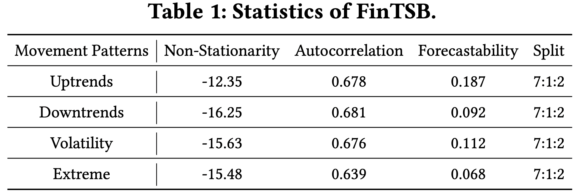
• All patterns exhibit strong non-stationarity

• Uptrend and downtrend patterns tend to exhibit higher autocorrelation

  \(\rightarrow\) Persistence of their directional movements

• Predictability of different movement patterns varies significantly

  • Uptrends and downtrends generally being more predictable

[3] Summary

• Encompasses a wide variety of sequence indicators
• Captures the multifaceted nature of FinTS
• Enables the exploration of diverse forecasting challenges

(2) Comparison Baselines

Covers the six categories of methods

• (1) Classic strategies: CSM [28], BLSW [51]
• (2) ML-based methods: XGBoost [6], LightGBM [30], DoubleEnsemble [2020], ARIMA [4]
• (3) DL-based methods: Linear, LSTM [22], ALSTM [52], GRU [10], GCN [31], GAT [59], TCN [3], Transformer [58], Mamba [18], PatchTST [47], Crossformer [76], iTransformer [43], AMD [24], PDF [11], Localformer [77].
• (4) RL-based methods: PPO [54], DDPG [36], SAC [19], DQN [5]
• (5) Generative-based methods: DDPM [21], DDIM [57], FactorVAE [15]
• (6) LLM-based methods: Timer [44], Time-MoE [55], Chronos [2]

(3) Evaluation Metrics

11 metrics (across 3 dimensions)

• a) Ranking (4 metrics)
  • [1] Information Coefficient (IC)
  • [2] Information Coefficient Information Ratio (ICIR)
  • [3] Rank Information Coefficient (RankIC)
  • [4] Rank Information Coefficient Information Ratio (RankICIR)
• b) Portfolio (5 metrics)
  • [5] Annualized Return Ratio (ARR)
  • [6] Annualized Volatility (AVol)
  • [7] Maximum Draw Down (MDD)
  • [8] Annualized Sharpe Ratio (ASR)
  • [9] Information Ratio (IR)
• c) Error (2 metrics)
  • [10] MSE
  • [11] MAE

a) Ranking Metrics

Assess the performance of “predicted ranking scores (returns) \(Y\)“

• Measure both cross-sectional and predictive power

[1] Information Coefficient (IC)

\(\mathrm{IC}=\frac{1}{N} \sum_{i=1}^N \frac{\sum_{k=1}^t\left(r_i^k-\bar{r}_i\right)\left(Y_i^k-\bar{Y}_i\right)}{\sqrt{\sum_{k=1}^t\left(r_i^k-\bar{r}_i\right)^2} \cdot \sqrt{\sum_{k=1}^t\left(Y_i^k-\bar{Y}_i\right)^2}}\).

• Goal: Quantifies the directional alignment between …
  • (1) Predicted \(Y\)
  • (2) GT \(r\)
• Metric: Spearman correlation coefficient
• Evaluates the raw predictive power of scores \(Y\)
  • Statistically significant positive IC values \(\rightarrow\) Meaningful forecasting power

[2] Information Coefficient Information Ratio (ICIR)

\(\mathrm{ICIR}=\frac{\text { mean }(\mathrm{IC})}{\operatorname{std}(\mathrm{IC})}\).

• Goal: Measures the stability of the performance of \(Y\)
• How: By comparing the annualized mean IC with its temporal volatility

[3] Rank Information Coefficient (RankIC)

\(\text { RankIC }=1-\frac{1}{N} \sum_{i=1}^N \frac{6 \sum_{k=1}^t\left(R\left(r_i^k\right)-R\left(Y_j^k\right)\right)^2}{t\left(t^2-1\right)}\), where \(R(\cdot)\) is the rank function.

• Goal: To eliminate scaling artifacts and reduces sensitivity to outlier bias

• How: Employs dual-ranking normalization

  \(\rightarrow\) Before calculating the correlation, both \(Y\) and \(r\) are converted to uniform percentile ranks

• Metric: Spearman correlation metric

[4] Rank Information Coefficient Information Ratio (RankICIR)

\(\text { RankICIR }=\frac{\text { mean }(\text { RankIC })}{\text { std(RankIC })}\).

• Goal: Evaluate the reliability of rank-based relationships between \(Y\) and \(r\).

b) Portfolio-Based Metrics

Evaluate the strategies through simulated portfolio implementation

[5] Annualized Return Ratio (ARR)

ARR \(=\) \((1+\text { Total Return })^{\frac{252}{n}}-1\)

• Primary indicator of strategy profitability
• Geometric mean return of a strategy annualized over the evaluation period

[6] Annualized Volatility (AVol)

\(\mathrm{AVol}=\sqrt{252 \cdot \operatorname{Var}\left(R_p\right)}\), where \(R_p\) denotes the daily return of the portfolio.

• Quantifies the dispersion of strategy returns

• Captures the consistency of performance delivery

  • Lower values \(\rightarrow\) More stable return streams

[7] Maximum Draw Down (MDD)

\[\mathrm{MDD}=-\max \left(\frac{p_{\text {peak }}-p_{\text {trough }}}{p_{\text {peak }}}\right)\]

• Represents the largest peak-totrough decline ( \(\left.p_{\text {peak }}-p_{\text {trough }}\right)\) over the evaluation period
• Critical in assessing the strategy’s risk tolerance

[8] Annualized Sharpe Ratio (ASR)

\(\mathrm{ASR}=\frac{\mathrm{ARR}}{\mathrm{AVol}}\).

• Measures the excess return per unit of total risk
• Assesses risk-adjusted performance

[9] Information Ratio (IR)

\(\mathrm{IR}=\frac{\operatorname{mean}\left(R_p-R_b\right)}{\operatorname{std}\left(R_p-R_b\right)}\), where \(R_b\) is the daily return of the market index

• Assesses the ability to generate excess returns relative to a benchmark

c) Error Metrics

( Note that a lower MSE or MAE does not guarantee profitability! )

\(\rightarrow\) Market impact, position sizing rules and transaction costs ultimately determine the success of the strategy!

• [10] \(\mathrm{MSE}=\frac{1}{L} \sum_{t=0}^L\left(Y_i^t-r_i^t\right)^2\).
• [11] \(\mathrm{MAE}=\frac{1}{L} \sum_{t=0}^L \mid Y_i^t-r_i^t \mid\).

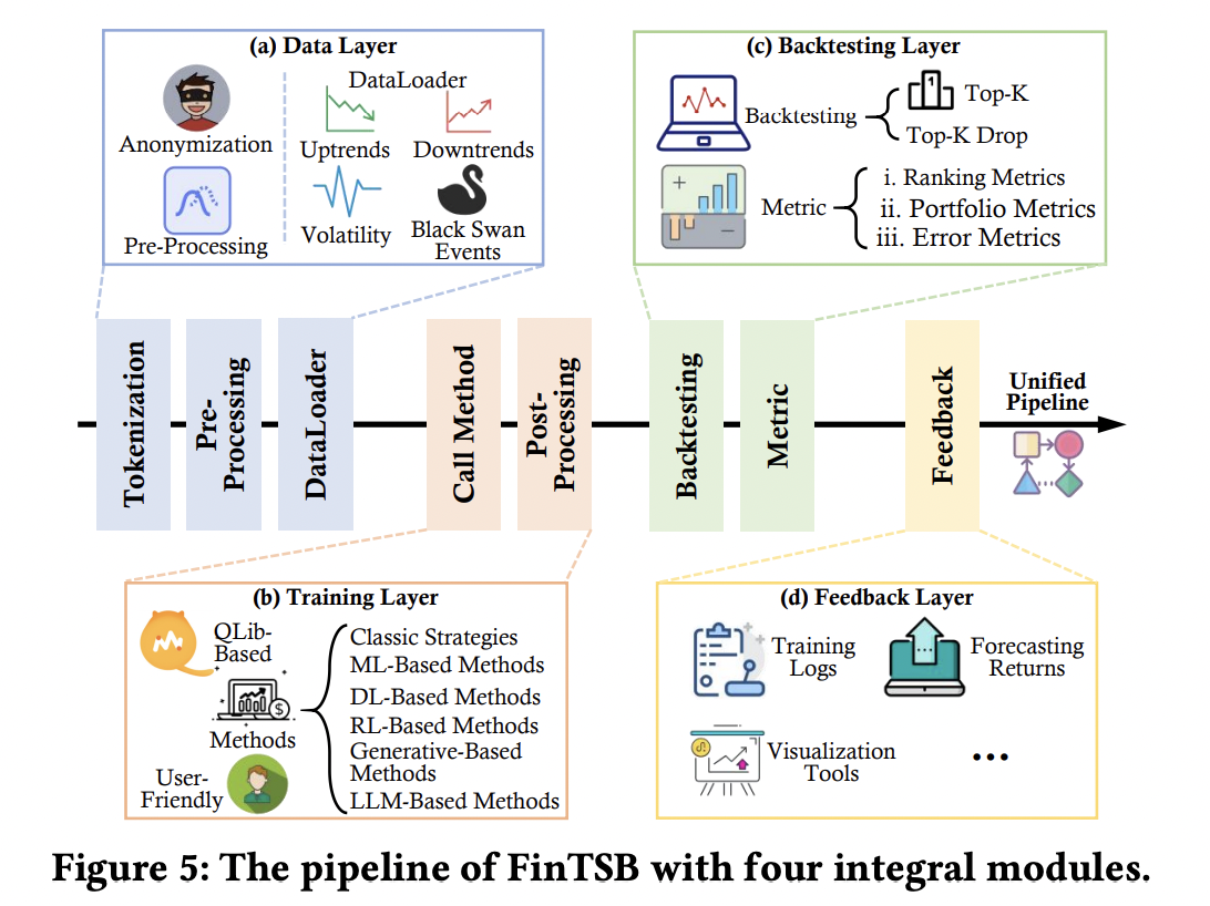
(4) Unified Pipeline

Divergent evaluation criteria

\(\rightarrow\) Differences in model performance!

How to ensure a fair, comprehensive, and practical evaluation?

\(\rightarrow\) Unified pipeline ,that is structurally divided into …

• (1) Data layer
• (2) Training layer
• (3) Backtesting layer
• (4) Feedback layer

a) Data Layer

• Comprehensive market information in FinTSB
• Four different movement patterns
• Data pre processing..
  • (1) Tokenization (anonymization)
  • (2) Normalization
• Dataloader
  • Dynamically constructs global training/validation/test sets based on the selected movement modes.
• Cross-pattern evaluation through transfer learning
  • Training on pattern A and testing on pattern B
  • Enables granular analysis of strategy adaptability across market regimes
  • For assessing model generalization capabilities.
• Historical stock market data verification
  • Validates model effectiveness in real-world financial scenarios

b) Training Layer

• Models built on six heterogeneous backbone architectures

• Easy-to-use and unified training pipeline

• Maintains model-agnostic compatibility

  \(\rightarrow\) Researchers employing FinTSF paradigm can seamlessly integrate their new models!

c) Backtesting Layer

• Two classic strategies:

  • (1) Top𝐾
  • (2) Top𝐾-Drop

  with transaction cost simulations reflecting real market conditions

• Comprehensively quantify model capabilities across 11 rigorously wide-used indicators.

d) Feedback Layer

• Archives training logs, preserves prediction results & Provides interactive visualization tools.
• Facilitates continuous model optimization by tracking performance across training iterations,

Summary

Users only need to deploy their method at the training layer & configuration file!

\(\rightarrow\) FinTSB can automatically run the pipeline!!

4. Experiments

(1) Experiment Setup

a) Resource

• A100: for LLM-based methods
• V100: for others

b) Hyperparameters

• \(L=20\), \(H=1\) ( Predict the returns \(Y\) on the next trading day )
• Hyperparameter searches across multiple sets for optimal results

c) Objective

\(\mathcal{L}=\frac{1}{L} \sum_{t=1}^L\left(\sum_{i=1}^N \mid \mid Y_i^t-r_i^t \mid \mid ^2+\eta \sum_{i=1}^N \sum_{j=1}^N \max \left(0,-\left(Y_i^t-Y_j^t\right)\left(r_i^t-r_j^t\right)\right)\right)\).

• Dual-objective optimization framework: Composite loss function that integrates both …

  • (1) Point-wise regression loss
  • (2) Pair-wise ranking loss

  ( with adaptive weighting coefficient \(\eta = 5\) )

(2) Trading Protocols

Top𝐾-Drop strategy

• Rather than fully rebalancing holdings daily…
• Retains stocks that persistently rank in the top-𝐾 cohort
• Only replaces underperformers

\(\rightarrow\) To maintain a portfolio on each trading day!

Advantages

• Improves upon Top𝐾 strategy by dynamically optimizing portfolio turnover

• Reduces the frequency of transactions

  \(\rightarrow\) Lowering commission costs in proportion to the actual turnover rate

• Maintains exposure to stocks with sustained high scores, avoiding unnecessary exits.

Mathematical expressions

• (On trading day \(t\)) Constructs an equal-weighted portfolio of \(m\) stocks \(\mathcal{P}^t=\left\{s_{i_1}^t, s_{i_2}^t, \ldots, s_{i_m}^t\right\}\)
  • which are selected according to the rank of predicted returns \(Y\)
• \(n\): Maximum number of change
  • Required to fulfill the condition \(\mid \mathcal{P}^t \cap \mathcal{P}^{t-1} \mid \geq m-n\).
• Experiments)
  • (1) Set \(m\) at one tenth of the total number of stocks, i.e., \(m=30\), and \(n\) is set to 5 .
  • (2) Transaction fee at a rate of \(0.1 \%\),

(3) Experimental Results

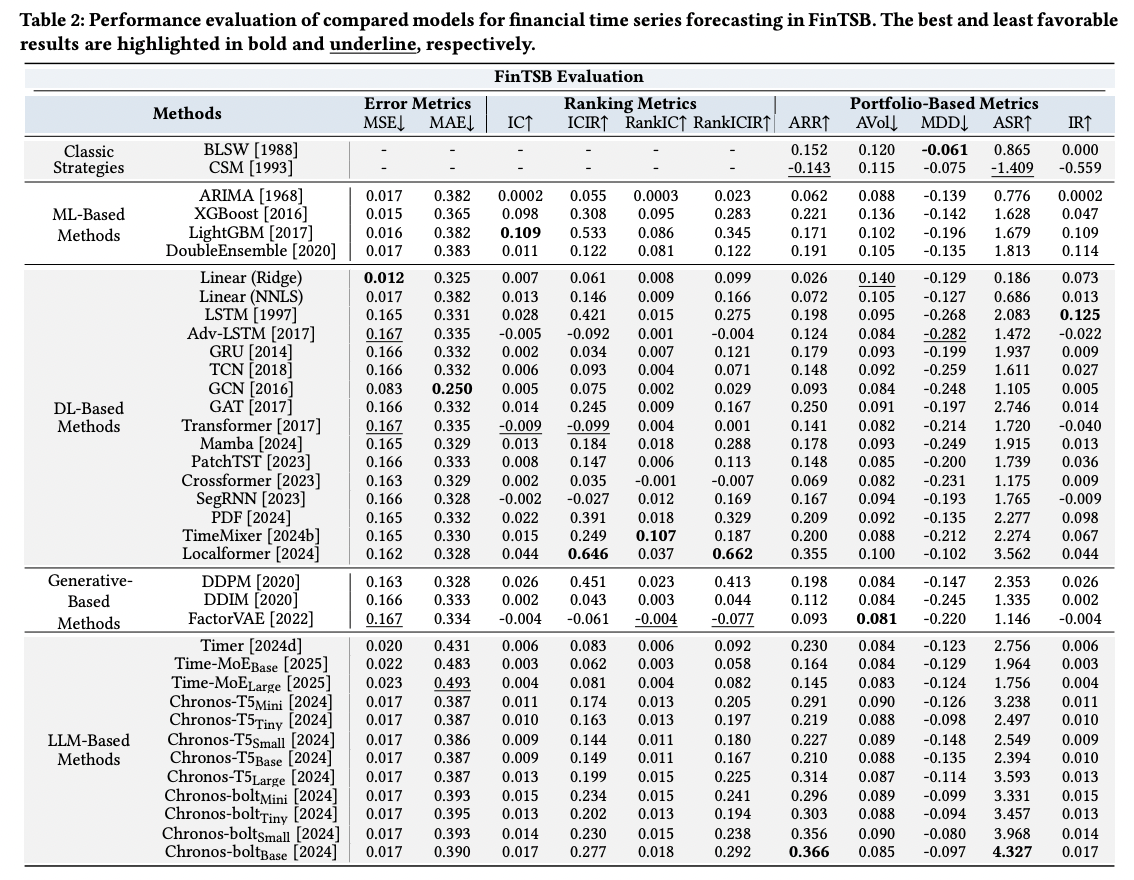
Summary

• (1) No universal best model!

  • No single method achieves the best performance across all three dimensional metrics!

• (2) Varies significantly even “within” same backbone

• (3) Emergent capabilities of LLM-based approaches

  • Performance initially deteriorates with model scaling, but subsequently shows marked improvement at larger scales.

    \(\rightarrow\) Possibly due to the need for sufficient parameters to disentangle complex market noise and latent factor interactions!

• (4) Modern DL

  • Do not universally outperform traditional quantitative strategies or tree-based models

\(\rightarrow\) Underscore the importance of considering both

• (1) Model scalability
• (2) FinTS characteristics

(4) Transfer Learning Results

To validate the cross-data generalization capability!

\(\rightarrow\) By applying models pretrained on FinTSB to backtest the entire 2024 CSI 300 stock market

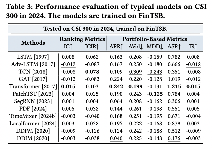
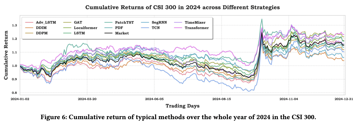
Two key insights

• (1) Model demonstrates remarkable performance consistency across different market regimes
• (2) Superior risk-adjusted returns achieved through this zero-shot transfer learning paradigm highlight FinTSB’s unique advantages in both pattern diversity coverage and temporal robustness, establishing it as a comprehensive benchmark for heterogeneous market behaviors spanning bull, bear, and transitional market phases.

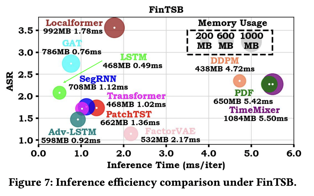
(5) Inference Efficiency

High demands on system latency sensitivity!

5. Conclusion

FinTSB = Comprehensive benchmark for FinTSF

Addresses three key challenges!