LLM-Mixer; Multiscale Mixing in LLMs for Time Series Forecasting

LLM-Mixer: Multiscale Mixing in LLMs for Time Series Forecasting

Contents

1. Abstract
2. Introduction
3. LLM-Mixer
4. Experiments

0. Abstract

LLM-Mixer

• Combiation of multiscale TS decomposition with pretrained LLMs

• Captures both

  • a) Short-term fluctuations

  • b) Long-term trends

    by decomposing data into multiple temporal resolutions

• Process them with frozen LLM (guided by textual prompt)

1. Introduction & Related Work

Challenges of “LLMs for TS forecasting”

• (1) Difference bewteen text vs TS

• (2) TS has “multiple time scales”

  • LLMs typically process fixed length seqeunces

    ( \(\rightarrow\) only capture short-term dependencies )

Solution: LLM-Mixer

• Breaks down TS into mulitple time scales

2. LLM Mixer

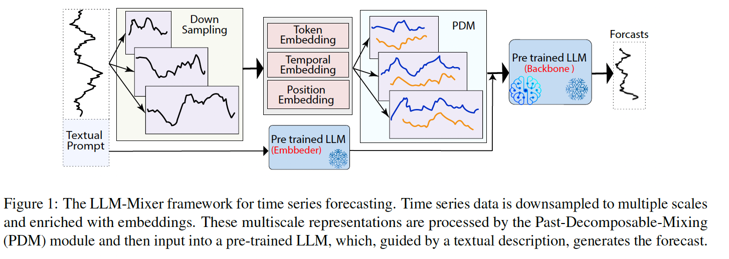
(1) Multi-scale View of Time Data

Apply multiscale mixing strategy

Procedure

• Step 1) Downsample into \(\tau\) scales
  • Result: multiscale representation \(\mathcal{X}=\left\{\mathbf{x}_0, \mathbf{x}_1, \ldots, \mathbf{x}_\tau\right\}\),
    • \(\mathbf{x}_i \in \mathbb{R}^{\frac{T}{2^2} \times M}\).
    • \(\mathbf{x}_0\) : the finest temporal details
    • \(\mathrm{x}_\tau\) : the broadest trends.
• Step 2) Project multiscale series with DNN
  • Token embedding
  • Temporal embedding
  • Positional Embedding
• Step 3) Stacked Past-Decomposable-Mixing (PDM) blocks
  • (For the \(l\)-th layer) \(\mathcal{X}^l=P D M\left(\mathcal{X}^{l-1}\right), \quad l \in L\)
    • \(\mathcal{X}^l=\) \(\left\{\mathbf{x}_0^l, \mathbf{x}_1^l, \ldots, \mathbf{x}_\tau^l\right\}\), with each \(\mathbf{x}_i^l \in \mathbb{R}^{\frac{T}{2^i} \times d}\),

(2) Prompt Embedding

Prompting

• Effective technique for guiding LLMs
• By using task-specific information

Use textual description for all samples in a dataset

\(\rightarrow\) Generate its embedding using pretrained LLM’s embedding \(E \in \mathbb{R}^{V \times d}\)

(3) Multi-scale Mixing in LLM

(After \(L\) PDM blocks) Obtain the multiscale past information \(\mathcal{X}^L\).

Result: \(\mathbb{F}\left(E \oplus \mathcal{X}^L\right)\).

Apply a trainable decoder (simple linear transformation) to the last hidden layer of the LLM

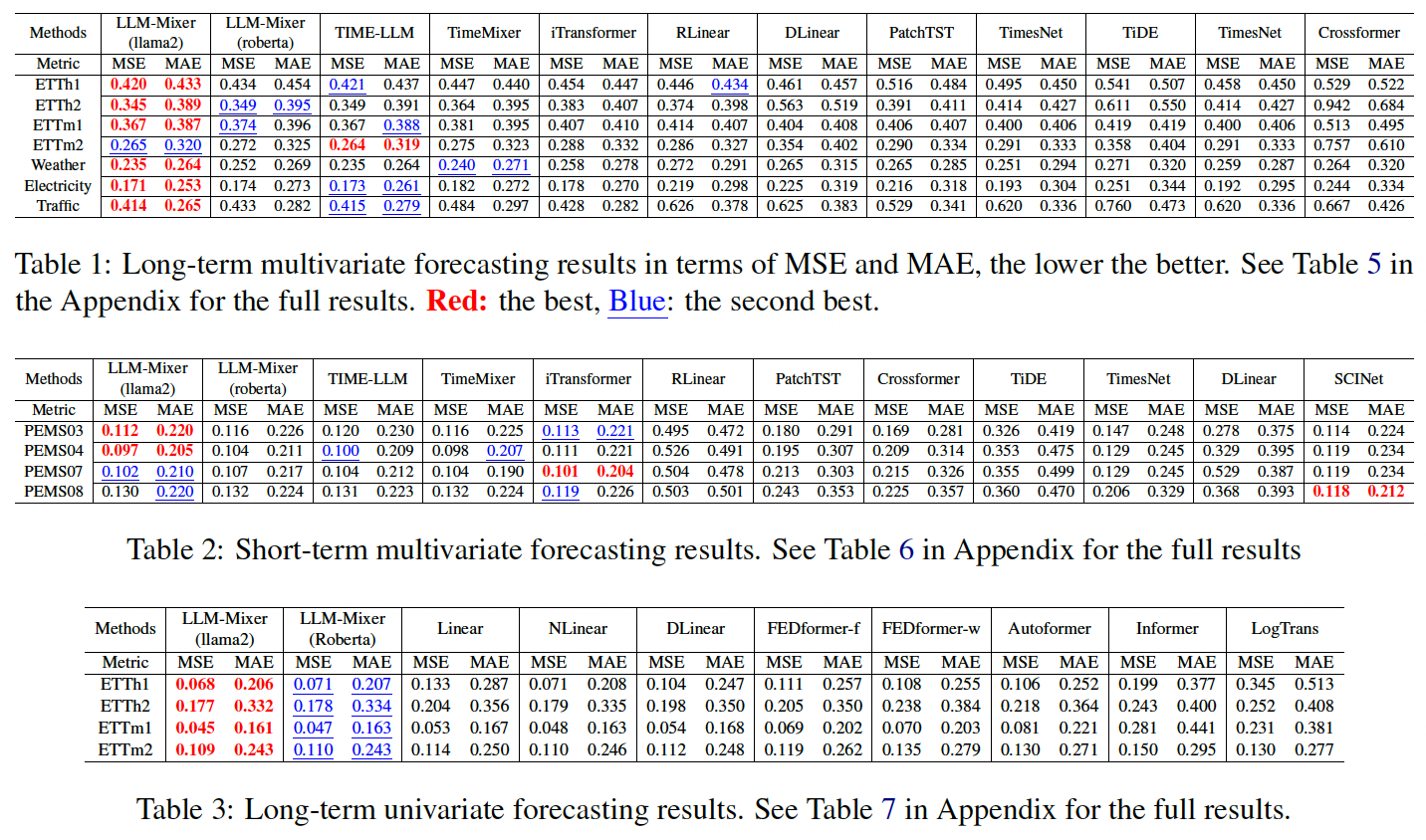
3. Experiments