LeMoLE; LLM-Enhanced Mixture of Linear Experts for Time Series Forecasting

LeMoLE: LLM-Enhanced Mixture of Linear Experts for Time Series Forecasting

Contents

1. Abstract
2. Introduction
3. Related Works
4. LeMoLE
5. Experiments

0. Abstract

Aligning TS into space of LLM: high computational cost

Proposal: LLM-enhanced mixture of linear experts

LeMoLE

• (1) Mixture of linear experts with multiple lookback length (\(L\))

  \(\rightarrow\) Efficient due to simplicity

• (2) Multimodal fusion mechanism

  \(\rightarrow\) Adaptively combines multiple linear experts based on the learned features of text modality

1. Introduction

(1) Trend 1: Linear model

• Have been outperforming in TS domain, while maintaining efficiency

• Nontheless, limitations:

  • (1) Non-linear patterns

  • (2) Long-range dependencies

\(\rightarrow\) Mixture of linear experts

• e.g., some focus on trend, some handle seasonalities …

Mixture-of-Linear-Experts (MoLE)

• Train multiple linear-centric models (i.e., experts) to collaboratively predict TS

• Router model

  • Accepts a timestamp embedding of input sequence as input

  • Learns to weight these experts adaptively

    \(\rightarrow\) Allows different experts specialize in different periods of TS

(2) Trend 2: Multimodal knowledge

Proposal: LeMoLE

LLM-enhanced mixture of linear experts

Difference with MoLE

• (1) Enhances ensemble diversity by leveraging experts with varying \(L\)s
  • handle both short & long term temporal patterns
• (2) Multimodal knowledge
  • From global & local text data
  • Allows LeMoLE to allocate specific experts for specific temporal patterns
• (3) Incorporate static & dynamic text information
  • Two conditioning moudles (based on FiLM, 2018)

Contributions

1. LeMoLE: based on (1) mixture-of-expert learning & (2) multimodal learning

2. Linear experts with varying \(L\) for diversity

   ( + incorporate 2 conditioning modules to effectively integrate global & local text info )

3. Rethinkg existing LLMs for TS

2. Related Works

(1) Linear Models

TimeMixer (2024)

• Mix the decomposed season & trend components from multiple resolution
• Multiple predictors

MoLE (2024)

• Multiple linear experst
• Based on a router module
  • to adaptively reweight experts’ output for final prediction
• (proposed) LeMoLE = MoLE + Multimodal fusion mechanism

(2) LLM-based Multimoal Forecasting

Main challenges: Misalignment in modalities

3. LeMoLE: LLM-Enhanced Mixture of Linear Experts

Problem Formulation

• Lookback window: \(\mathbf{X}_{1: T} \in \mathbb{R}^{T \times C}\)

• Forecast window: \(\mathbf{X}_{T+1: T+H}\)

• Model: \(\mathbf{X}_{T+1: T+H}=\mathcal{F}^*\left(\mathbf{X}_{1: T}\right)\)

• Prompts:
  • Static prompt: \(\mathbf{P}_S\)
  • Dynamic prompt: \(\mathbf{P}_D\)
• Model with prompts: \(\hat{\mathbf{X}}_{T+1: T+H}=\mathcal{F}\left(\mathbf{X}_{1: T}, \mathbf{P}_D, \mathbf{P}_S\right)\).

Overall Architecture

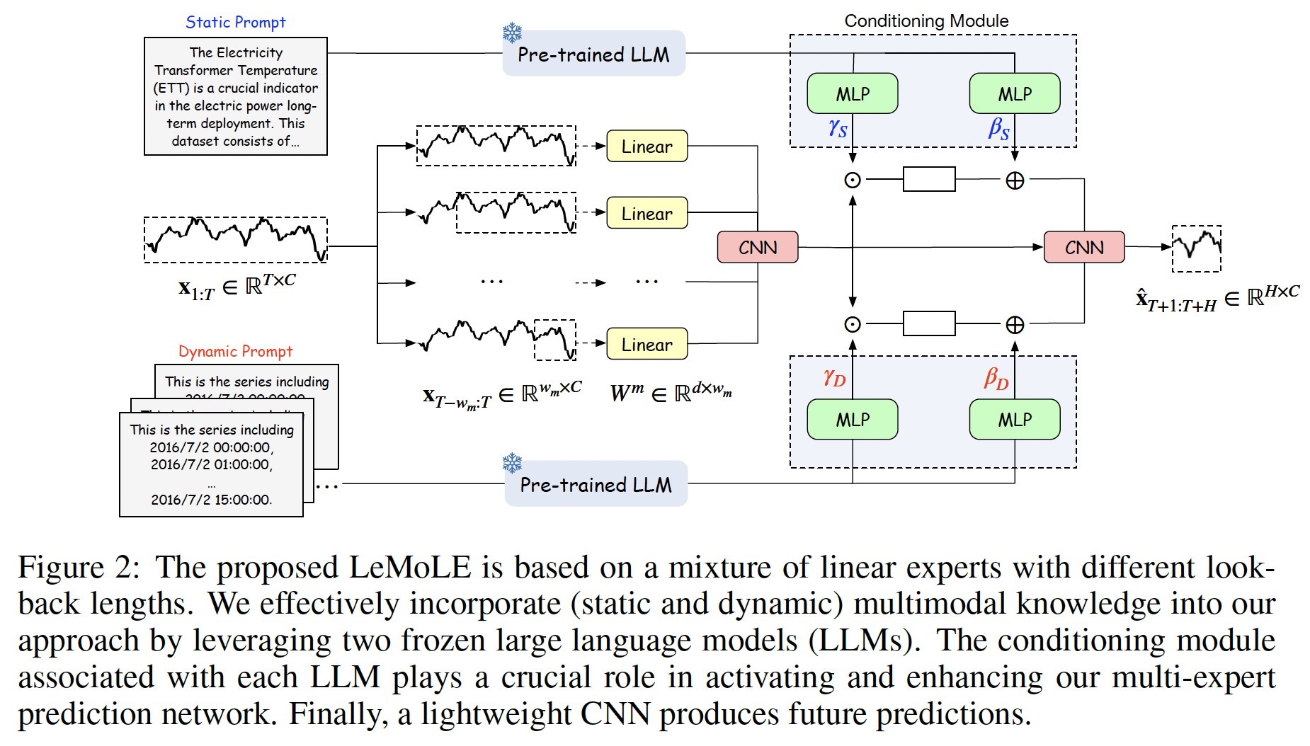
(1) MoLE

\(\mathbf{Y}^{(m)}=\mathbf{W}_m \mathbf{X}_{T-w_m: T}+\mathbf{b}_m,\).

• where \(m=1, \ldots, M\)
• \(\mathbf{W}_m \in \mathbb{R}^{H \times w_m}\) and \(\mathbf{b}_m \in \mathbb{R}^{H \times C}\) are trainable expert-specific parameters.

Obtain \(M\) prediction output from \(M\) linear experts

\(\rightarrow\) Denoted by \(\left\{Y^{(1)}, Y^{(2)}, \ldots, Y^{(M)}\right\}\).

(2) LLM-enhanced Conditioning Module

For prompting, essential to design ..

• a) Appropriate text prompts
• b) Corresponding conditioning module to activate the multi-expert prediction network

TS data: two types of text info

• (1) Static text
  • Global information about TS
  • e.g., Data source description
• (2) Dynamic text ( time-dependent )
  • Local information about TS
  • e.g., time stamps, weather conditions ..

a) Static prompt \(\mathbf{P}_S\)

\(\mathbf{P}_S\) = Contains the \(L_S\) length of texts (including punctuation marks)

\(\mathbf{Z}_S=\mathcal{L} \mathcal{L M}\left(\mathbf{P}_S\right)\).

• Text representation vector \(\mathbf{Z}_S \in \mathbb{R}^{L_S \times d_{l l m}}\),

b) Dynamic prompt \(\mathbf{P}_D\)

Timestamps in the datasets

• Follow AutoTimes (Liu et al., 2024b) to use the timestamps as related dynamic text data

Aggregate textual covariates \(\mathbf{T}_{T-w_1}, \ldots, \mathbf{T}_T\) to generate the dynamic prompt as \(\mathbf{P}_D \in \mathbb{R}^{L_D \times 1}\).

\(\mathbf{P}_D=\operatorname{Prompt}\left(\left[\mathbf{T}_{T-w_1}, \mathbf{T}_{T-w_1+1}, \ldots, \mathbf{T}_T\right]\right)\),

\(\mathbf{Z}_D=\mathcal{L} \mathcal{L} \mathcal{M}\left(\mathbf{P}_D\right)\).

(3) Conditioning Module

Use the prompts as conditions to activate our multi-expert prediction network.

• \(\mathbf{Z}_S \in \mathbb{R}^{L_S \times d_{U m}}\) and \(\mathbf{Z}_D \in \mathbb{R}^{L_D \times d_{U m}}\)

Two conditioning modules

• To fuse \(\mathbf{Z}_S\) and \(\mathbf{Z}_D\) respectively
• Based on the popular conditioning layer, FiLM (Perez et al., 2018)
  • Use a CNN to map the multi-linear experts’ outputs \(\left\{\mathbf{Y}^{(1)}, \mathbf{Y}^{(2)}, \ldots, \mathbf{Y}^{(M)}\right\}\)
  • \(\mathbf{Y}=\operatorname{CNN}\left(\left[\mathbf{Y}^{(1)} ; \mathbf{Y}^{(2)} ; \ldots ; \mathbf{Y}^{(M)}\right]\right)\).
  • Step 1) \(\mathbf{Y}_S^{\prime}=\gamma_S \odot \mathbf{Y}+\beta_S\)
  • Step 2) \(\mathbf{Y}_D^{\prime}=\gamma_D \odot \mathbf{Y}+\beta_D\)

Final prediction

• Light-weight CNN blocks to summarize all branches
• \(\hat{\mathbf{Y}}=\operatorname{CNN}^{\mathrm{final}}\left(\left[\mathbf{Y} ; \mathbf{Y}_S^{\prime} ; \mathbf{Y}_D^{\prime}\right]\right)\).

Loss function: \(\mathcal{L}= \mid \mid \mathbf{x}_{T+1: T+H}-\hat{\mathbf{Y}} \mid \mid _2^2\).

4. Experiments