(paper) Deep Learning For Time Series Classification

Deep Learning For Time Series Classification (2018, 1191)

Contents

1. Introduction

2. SOTA of TSC

   1. Background
   2. DL for TSC
   3. Generative / Discriminative approaches

3. Benchmarking DL for TSC

   ( 9 methods )

0. Introduction

Tasks

• 1) forecasting
• 2) anomaly detection
  • time series outlier detection
  • common application : predictive maintenance
    • ex) predicting anomalies in advance, to prevent potential failures
• 3) clustering
  • ex) discovering daily patterns of sales in Marketing DB
• 4) classification
  • data point itself is a “whole time series”

Review about TSC with DL

• different techniques to improve accuracy
  • ex) regularization / generalization capabilities
    • transfer learning
    • ensembling
    • data augmentation
    • adversarial training
• test on dataset…
  • UCR/UEA archive ( 85 univariate TS )

2. SOTA of TSC

Question :

• Q1) SOTA DNN for TSC?
• Q2) Approach that reaches SOTA, less complicated than HIVE-COTE?
• Q3) How does random initialization affect performance?
• Q4) How about Interpretability?

(1) Background

Notation

• \(X=\left[x_{1}, x_{2}, \ldots, x_{T}\right]\) : univariate

• \(X=\left[X^{1}, X^{2}, \ldots, X^{M}\right]\) : multivariate

  • # of dimension : \(M\)

  • \[X^{i} \in \mathbb{R}^{T}\]

• \(D=\left\{\left(X_{1}, Y_{1}\right),\left(X_{2}, Y_{2}\right), \ldots,\left(X_{N}, Y_{N}\right)\right\}\) : dataset

  • \(X_{i}\) : could either be a univariate or multivariate
  • \(Y_{i}\) : one-hot label vector ( \(K\) classes )

(2) DL for TSC

Focus on 3 main DNN architetures

• 1) MLP
• 2) CNN
• 3) ESN

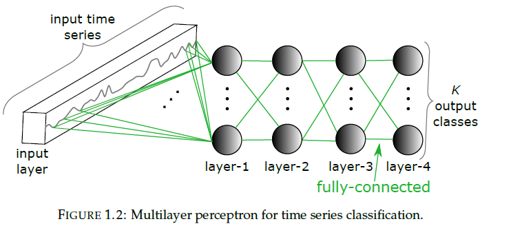
(a) MLP

• input neuron : \(T \times M\) values

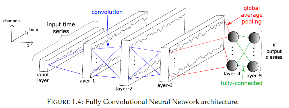
(b) CNN

• result of convolution on \(X\) can be considered as “another univariate TS” \(C\)
• thus, applying several filters \(\rightarrow\) MTS!
• unlike MLP, share weights!
• # of filters = # of dimension in MTS
• Pooling
  • local pooling : average/max
  • global pooling : TS will be aggregated over “whole” TS, resulting in single value
    • drastically reduce parameters
• Normalization
  • quick convergence
• Batch normalization
  • prevent internal covariance shift

(c) ESN

RNN : not widely used for TSC, due to…

• 1) designed mainly to “predict an output for EACH ELEMENT”
• 2) vanishing gradient problem
• 3) hard to train & parallelize

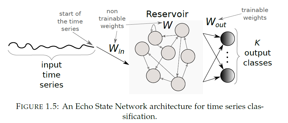
ESNs (Echo State Networks) :

• mitigate challenges of RNNs, by eliminating the need to compute the gradient of hidden layers

  \(\rightarrow\) reduces training time

• sparsely connected random RNN

(3) Generative / Discriminative approaches

(a) Generative

pass

(b) Discriminative

feature extraction methods

• ex) transform TS to image!
  • 1) Gramian fields
  • 2) Reccurence Plots
  • 3) Markov Transition Fields

in contrast to feature engineering…“End-to-End” DL

• incorporate feature learning process!

2. Benchmarking DL for TSC

limit experiment to “End-to-End Discriminative DL models for TSC”

\(\rightarrow\) chose 9 approaches

(1) MLP

pass

(2) FCNs

pass

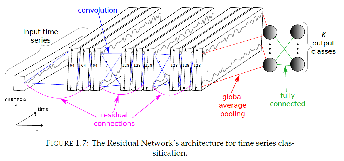
(3) Residual Network

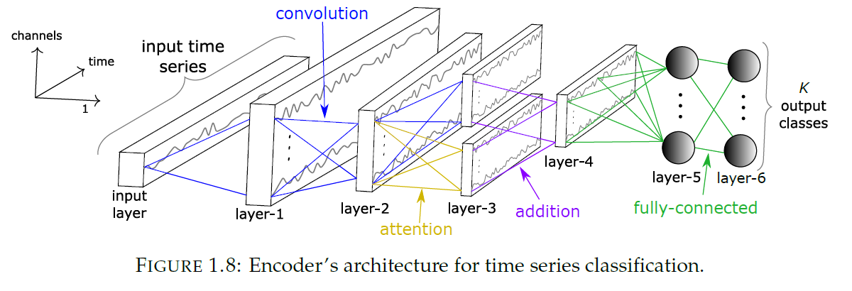
(4) Encoder

2 variants

• 1) train from scratch ( end-to-end )
• 2) use pre-trained model & fine-tune

3 layers are convolutional

replace GAP to attention

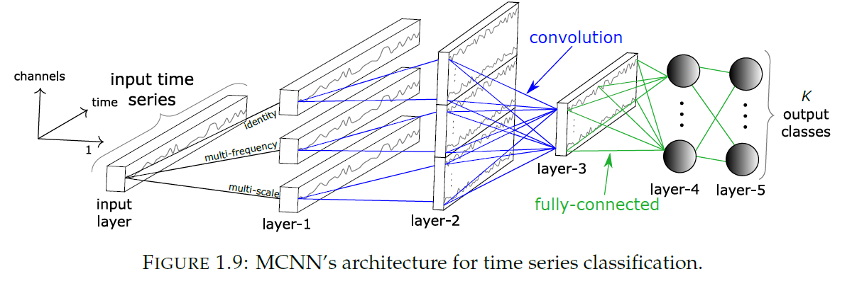
(5) MCNN ( Multi-scale CNN )

very similar to traditional CNN

but, very complex with its “heavy data preprocessing step”

• step 1) WS method as data augmentation

  • slides a window over input TS

• step 2) transformation stage

  • a) identity mapping
  • b) down sampling
  • c) smoothing

  “transform UNIVARIATE to MULTIVARIATE”

class label is determined by majority vote over extracted subsequences!

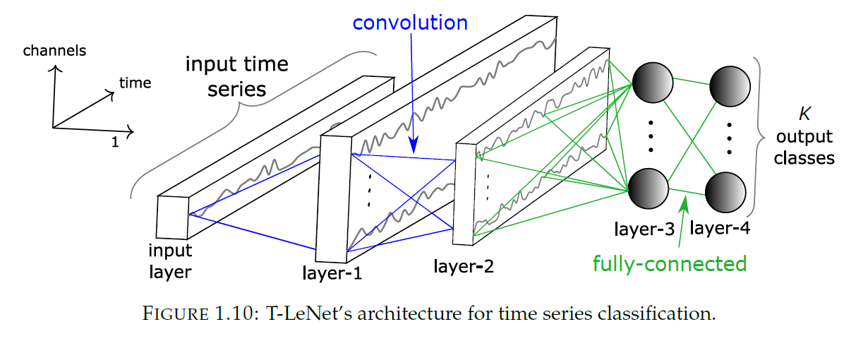
(6) Time Le-Net

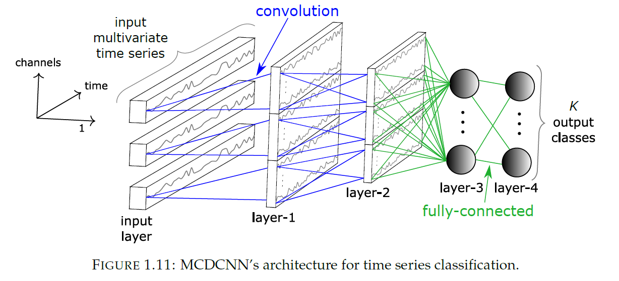
(7) MCDCNN ( Multi Channel Deep CNN )

traditional CNN + MTS

• convolutions are applied “independently (in parallel)” on each dimension

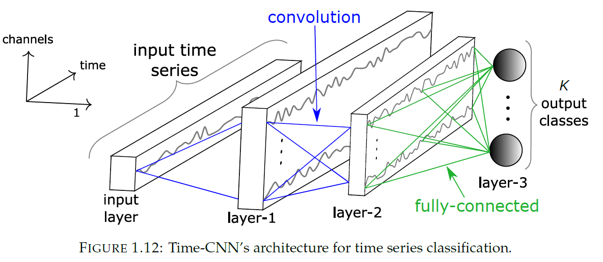
(8) Time-CNN ( Time Convolutional Neural Network )

for both “UNI-variate” & “MULTI-variate”

use MSE, instead of CE

• \(K\) output nodes ( with sigmoid activation function )

(9) TWIESN ( Time Warping Invariant Echo State Network )

pass