64.Wasserstein Variational Inference (NeurIPS 2018)

Wasserstein Variational Inference (NeurIPS 2018)

Abstract

• Introduce Wasserstein Variational Inference ( = Bayesian Inference based on optimal transport theory )

• Uses a new family of divergence, which includes (1) f-divergence & (2) Wasserstein distance

• Gradients of Wasserstein variational loss : obtained by backpropagating through the Sinkhorn iterations

• Introduce several new forms of autoencoders

1. Introduction

in Variational Inference … KL divergence plays the central role

But recently, OPTIMAL TRANSPORT DIVERGENCES such as Wasserstein distance have gained popularity

• usually in “generative modeling”

  \(\because\) well-behave in situations where KL-divergence is either infinite or undefined

Proposes variational Bayesian inference! define new c-Wasserstein family of divergences

• includes (1) f-divergence & (2) Wasserstein distance
  • f-divergences include both “forward & reverse KL”

1-1. Background on joint-contrastive variational inference

Review about joint-contrastive variational inference

• latent variable \(z\)
• observed data \(x\)

ex) reverse KL-divergence : \(D_{K L}(p(x, z) \mid \mid q(x, z))=\mathbb{E}_{q(x, z)}\left[\log \frac{q(x, z)}{p(x, z)}\right]\)

• \(q(x, z)=q(z \mid x) k(x)\) : product between the variational posterior & sampling distribution of the data.
• advantage : no need to evaluate the intractable distn \(p(z \mid x)\)

1.2 Background on optimal transport

(1) Optimal transport divergences :

• distance between two probability distns as the cost of transporting probability mass from one to the other.

• \(\Gamma[p, q]\) : set of all bivariate probability measures on the product space \(X \times X\), whose marginals are \(p\) and \(q\)

• formula :

  \(W_{c}(p, q)=\inf _{\gamma \in \Gamma[p, q]} \int c\left(x_{1}, x_{2}\right) \mathrm{d} \gamma\left(x_{1}, x_{2}\right)\).

  • super-cubic complexity
  • complexity can be reduced by adopting “entropic regularization”

(2) Define new set of joint distn

• \(U_{\epsilon}[p, q]=\left\{\gamma \in \Gamma[p, q] \mid D_{K L}(\gamma(x, y) \mid \mid p(x) q(y)) \leq \epsilon^{-1}\right\}\).
  • have the “mutual info” between two variables, bounded by the regularization param \(\epsilon^{-1}\)

(3) Rewrite optimal transport divergence using above :

• \(W_{c, \epsilon}(p, q)=\inf _{u \in U_{\epsilon}[p, q]} \int c\left(x_{1}, x_{2}\right) \mathrm{d} u\left(x_{1}, x_{2}\right)\).

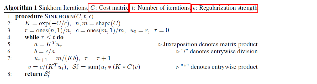
• when \(p\) and \(q\) are discrete distn : (by Sinkhorn iterations)

  \(W_{c, \epsilon}(p, q)=\lim _{t \rightarrow \infty} \mathcal{S}_{t}^{\epsilon}[p, q, c]\).

  • \(\mathcal{S}_{t}^{\epsilon}[p, q, c]\) : output of the \(t^{th}\) Sinkhorn iteration

2. Wasserstein Variational Inference

(1) introduce new family of divergences, includes both (1) optimal transport divergences & (2) f-divergences

(2) Then, develop a black-box and likelihood-free variational algorithm

2-1. c-Wasserstein divergences

(1) Traditional divergences

• ex) KL-divergence
• depend explicitly on the distn \(p\) and \(q\)

(2) Optimal transport divergences

• ex) Wasserstein distance
• depend on the distn \(p\) and \(q\) only through the constraints of an optimization problem

(1)+(2) = New divergence, “c-Wasserstein divergence”

• generalize both forms of dependencies ( (1) and (2) )
• FORMULA : \(W_{C}(p, q)=\inf _{\gamma \in \Gamma[p, q]} \int C^{p, q}\left(x_{1}, x_{2}\right) \mathrm{d} \gamma\left(x_{1}, x_{2}\right)\).

\(W_{C}(p, q)=\inf _{\gamma \in \Gamma[p, q]} \int C^{p, q}\left(x_{1}, x_{2}\right) \mathrm{d} \gamma\left(x_{1}, x_{2}\right)\)>

• cost function \(C^{p, q}\left(x_{1}, x_{2}\right)\) :

  • depends both on the 2 scalars \(x_{1}\) and \(x_{2}\) and on 2 distributions \(p\) and \(q\)

  • assumes to following properties :

    \(\begin{array}{l} \text { 1. } C^{p, p}\left(x_{1}, x_{2}\right) \geq 0, \forall x_{1}, x_{2} \in \operatorname{supp}(p) \\ \text { 2. } C^{p, p}(x, x)=0, \forall x \in \operatorname{supp}(p) \\ \text { 3. } \mathbb{E}_{\gamma}\left[C^{p, q}\left(x_{1}, x_{2}\right)\right] \geq 0, \forall \gamma \in \Gamma[p, q] \end{array}\).

    
    

[ Theorem 1 ]

The functional \(W_{C}(p, q)\) is a (pseudo-)divergence, meaning that \(W_{C}(p, q) \geq 0\) for \(p\) and \(q\) and \(W_{C}(p, p)=0\) for all \(p\)

• all optimal transport divergences are part of” “c-Wasserstein family”

[ Theorem 2 ]

Let \(f: \mathbb{R} \rightarrow \mathbb{R}\) be a convex function such that \(f(1)=0 .\) The cost functional \(C^{p, q}(x, y)=f(g(x, y))\) respects property 3 when \(\mathbb{E}_{\gamma}[g(x, y)]=1\) for all \(\gamma \in \Gamma[p, q]\)

[ Theorem 3 ]

Let \(W\left(p_{n}, q_{n}\right)\) be the Wasserstein distance between two empirical distributions \(p_{n}\) and \(q_{n}\).

For \(n\) tending to infinity, there is a positive number s such that \(\mathbb{E}_{p q}\left[W\left(p_{n}, q_{n}\right)\right] \lesssim W(p, q)+n^{-1 / s}\)

2.2 Stochastic Wasserstein variational inference

( loss func ) c-Wasserstein divergence between \(p(x, z)\) and \(q(x, z)\) :

\(\mathcal{L}_{C}[p, q]=W_{C}(p(z, x), q(z, x))=\inf _{\gamma \in \Gamma[p, q]} \int C^{p, q}\left(x_{1}, z_{1} ; x_{2}, z_{2}\right) \mathrm{d} \gamma\left(x_{1}, z_{1} ; x_{1}, z_{1}\right)\)……… eq(A)

• minimized when \(p=q\)
• but \(\mathcal{L}_{C}[p, q]\) could be 0 even if \(p \neq q .\)

Black-box MC estimate of the gradient of eq(A) :

• step 1) discrete c-Wasserstein divergence

  \[\mathcal{L}_{C}\left[p_{n}, q_{n}\right]=\inf _{\gamma} \sum_{j, k} C^{p, q}\left(x_{1}^{(j)}, z_{1}^{(j)}, x_{2}^{(k)}, z_{2}^{(k)}\right) \gamma\left(x_{1}^{(j)}, z_{1}^{(j)}, x_{2}^{(k)}, z_{2}^{(k)}\right)\]
  • where \(\left(x_{1}^{(j)}, z_{1}^{(j)}\right)\) and \(\left(x_{2}^{(k)}, z_{2}^{(k)}\right)\) are sampled from \(p(x, z)\) and \(q(x, z)\) respectively
  • asymptotically unbiased

• step 2) use the modified loss ( to eliminate bias )

  \(\tilde{\mathcal{L}}_{C}\left[p_{n}, q_{n}\right]=\mathcal{L}_{C}\left[p_{n}, q_{n}\right]-\left(\mathcal{L}_{C}\left[p_{n}, p_{n}\right]+\mathcal{L}_{C}\left[q_{n}, q_{n}\right]\right) / 2\).

  • expectation = 0 ( when \(p=q\) )

    \(\lim _{n \rightarrow \infty} \tilde{\mathcal{L}}_{C}\left[p_{n}, q_{n}\right]=\mathcal{L}_{C}[p, q]\).

• step 3) compute the gradient of the loss ( using automatic differentiation )

  entropy-regularized version of optimal transport cost can be approximated by truncating the Sinkhorn iterations

  \(\nabla \mathcal{L}_{C}\left[p_{n}, q_{n}\right]=\nabla \mathcal{S}_{t}^{\epsilon}\left[p_{n}, q_{n}, C_{p, q}\right]\).

3. Examples of c-Wasserstein divergences

now introduce 2 classes of c-Wasserstein divergences

• that are suitable for deep Bayesian VI
• question : how to define COST?

Show that KL-div & f-div are part of c-Wasserstein divergences

3-1. (1) A metric divergence for latent space

cost : \(C_{P B}^{p}\left(z_{1}, z_{2}\right)=d_{x}\left(g_{p}\left(z_{1}\right), g_{p}\left(z_{2}\right)\right)\)

• simplest way to assign a geometric transport cost to the latent space :

  pull back a metric function from the observable space

• \(d_{x}\left(x_{1}, x_{2}\right)\) = metric function in the observable space

• \(g_{p}(z)\) = deterministic function that maps \(z\) to the expected value of \(p(x \mid z)\)

3.2 (2) Autoencoder divergences

(1) Latent autoencoder cost

cost : \(C_{L A}^{q}\left(x_{1}, z_{1} ; x_{2}, z_{2}\right)=d\left(z_{1}-h_{q}\left(x_{1}\right), z_{2}-h_{q}\left(x_{2}\right)\right)\)

• ( expected value of \(q(z \mid x)\) is given by the deterministic function \(h_q(z)\) )
• transport cost between the latent residuals of the two models

(2) Observable autoencoder cost

cost : \(C_{O A}^{p}\left(x_{1}, z_{1} ; x_{2}, z_{2}\right)=d\left(x_{1}-g_{p}\left(z_{1}\right), x_{2}-g_{p}\left(z_{2}\right)\right)\).

• \(g_{p}(z)\) gives the expected value of the generator

• if deterministic generator :

  • \(C_{O A}^{p}\left(x_{1}, z_{1} ; x_{2}, z_{2}\right)=d\left(0, x_{2}-g_{p}\left(z_{2}\right)\right)\).

  • then, the resulting divergence is just “average reconstruction error”

    \(\inf _{\gamma \in \Gamma[p]} \int d\left(0, x_{2}-g_{p}\left(z_{2}\right)\right) \mathrm{d} \gamma=\mathbb{E}_{q(x, z)}\left[d\left(0, x-g_{p}(z)\right)\right]\).

  
  

3-3. \(f\)- divergences

all \(f\)-divergences are part of c-Wasserstein family!

cost : \(C_{f}^{p, q}\left(x_{1}, x_{2}\right)=f\left(\frac{p\left(x_{2}\right)}{q\left(x_{2}\right)}\right)\).

• \(f\) : convex function such that \(f(0)=1\)

• by [ Theorem 2 ], it defines a valid c-Wasserstein divergence

  
  

4. Wasserstein Variational Autoencoders

Notation

• \(\mathcal{D}_{p}\) and \(\mathcal{D}_{q}\) : parametrized probability distributions

• \(g_{p}(z)\) and \(h_{q}(x)\) : outputs of deep networks

Decoder (probabilistic model) : \(p(z, x)=\mathcal{D}_{p}\left(x \mid g_{p}(z)\right) p(z)\).

Encoder (variational model) : \(q(z, x)=\mathcal{D}_{q}\left(z \mid \boldsymbol{h}_{q}(x)\right) k(x)\)

Define a LARGE family of objective functions of VAEs by combining costs functions!

​ \(\begin{aligned} C_{\boldsymbol{w}, f}^{p, q}\left(x_{1}, z_{1} ; x_{2}, z_{2}\right)=& w_{1} d_{x}\left(x_{1}, x_{2}\right)+w_{2} C_{P B}^{p}\left(z_{1}, z_{2}\right)+w_{3} C_{L A}^{p}\left(x_{1}, z_{1} ; x_{2}, z_{2}\right) \\ &+w_{4} C_{O A}^{q}\left(x_{1}, z_{1} ; x_{2}, z_{2}\right)+w_{5} C_{f}^{p, q}\left(x_{1}, z_{1} ; x_{2}, z_{2}\right) \end{aligned}\).

5. Connections with related methods

5-1. Operator Variational Inference (?)

Wasserstein Variational Inference = “special case of generalized version of operator variational inference”

operator variational inference

• objective : \(\mathcal{L}_{O P}=\sup _{f \in \mathfrak{F}} \zeta\left(\mathbb{E}_{q(x, z)}\left[\mathcal{O}^{p, q} f\right]\right)\).

• [ dual representation ]

  c-Wasserstein loss : \(W_{c}(p, q)=\sup _{f \in L_{C}}\left[\mathbb{E}_{p(x, z)}[f(x, z)]-\mathbb{E}_{q(x, z)}[f(x, z)]\right]\)

  ​ where \(L_{C}[p, q]=\left\{f: X \rightarrow \mathbb{R} \mid f\left(x_{1}, z_{1}\right)- f\left(x_{2}, z_{2}\right) \leq C^{p, q}\left(x_{1}, z_{1} ; x_{2}, z_{2}\right)\right\}\)

• using importance sampling…

  \(W_{c}(p, q)=\sup _{f \in L_{C}[p, q]}\left[\mathbb{E}_{q(x, z)}\left[\left(\frac{p(x, z)}{q(x, z)}-1\right) f(x, z)\right]\right]\).

  
  

5-2. Wasserstein Autoencoders (WAE)

recently inroduced WAE : uses “regularized optimal transport divergence between \(p(x)\) and \(k(x)\)”

Regularized Loss : \(\mathcal{L}_{W A}=\mathbb{E}_{q(x, z)}\left[c_{x}\left(x, g_{p}(z)\right)\right]+\lambda D(p(z) \mid \mid q(z))\).

• derived from optimal transport loss!

  ( \(\mathcal{L}_{W A} \approx W_{c_{x}}(p(x), k(x))\) )

• when \(D(p(z) \mid \mid q(z))\) is c-Wasserstein divergence , \(\mathcal{L}_{W A}\) is a Wasserstein variational loss

  \(\mathbb{E}_{q(x, z)}\left[c_{x}\left(x, g_{p}(x)\right)\right]+\lambda W_{C_{z}}(p(z), q(z))=\inf _{\gamma \in \Gamma[p, q]} \int\left[c_{x}\left(x_{2}, g_{p}\left(z_{2}\right)\right)+\lambda C_{z}^{p, q}\left(z_{1}, z_{2}\right)\right] \mathrm{d} \gamma\).