
Hamiltonian Variational Auto-Encoder (NeurIPS 2018)
Abstract
VAEs : popular in “inference & learning latent variable models” ( combined with SVI.. “scalable” )
but for practical efficiency… necessary to obtain “low-variance” unbiased estimates of ELBO & its gradients
use of HMC has been suggested to achieve this, but not amenable to reparam trick
Suggest “Hamiltonian Importance Sampling (HIS)”
- optimally select reverse kernels
- allows to develop Hamiltonian Variational Autoencoder (HVAE)
1. Introduction
MFVI…can limit its flexibility
\(\rightarrow\) recent work : sampling from VAE posterior & transform these through mappings! Thus, richer posterior approximation!
( ex. Normalizing Flows )
Nfs have succeeded in various domains, but flows do not explicitly use informations about the target posterior!
- \(\therefore\) unclear whether the improved performance is caused by “accurate posterior” or “simply by overparameterization”
Hamiltonian Variational Inference (HVI)
-
stochastically evolves the base samples according to HMC ( thus use target information )
-
but relies on defining reverse dynamics in the flow
( turns out to be unnecessary )
Markov chain Monte Carlo and variational inference: Bridging the gap (2015
- possible to use \(K\) MCMC iterations to obtain an unbiased estimator of the ELBO and its gradients
- this estimator is obtained using importance sampling
- importance distn = joint distn of \(K+1\) states of “forward” Markov chain
- augmented target distn = constructed using “reverse” Markov kernels
- performance of estimator strongly depends on “forward & reverse kernels”
Hamiltonian dynamics
-
uses reverse kernels which are optimal for REDUCING VARIANCE of likelihood estimators
-
easily use the reparam trick
-
HVAE can be thought of as NFs, which the flow depends explicitly on the target distn
2. ELBO, MCMC, HIS
2-1. Unbiased Likelihood & ELBO
**(1) Likelihood function : **
-
\(p_{\theta}(x)=\int p_{\theta}(x, z) d z=\int p_{\theta}(x \mid z) p_{\theta}(z) d z\).
(2) under strictly positive unbiased estimate of \(p_{\theta}(x)\) :
-
\(\int \hat{p}_{\theta}(x) q_{\theta, \phi}(u \mid x) d u=p_{\theta}(x)\).
(3) ELBO of (2)
- \(\mathcal{L}_{\mathrm{ELBO}}(\theta, \phi ; x):=\int \log \hat{p}_{\theta}(x) q_{\theta, \phi}(u \mid x) d u \leq \log p_{\theta}(x)=: \mathcal{L}(\theta ; x)\).
- \(\mid \mathcal{L}_{\mathrm{ELBO}}(\theta, \phi ; x)-\mathcal{L}(\theta ; x)\mid\) decreases as the variance of \(\hat{p}_{\theta}(x)\) decreases
(4) Importance Weighted Auto-Encoder ( IWAE )
- ( Standard VI )
- \(\mathcal{U}=\mathcal{Z}\).
- \(\hat{p}_{\theta}(x)=p_{\theta}(x, z) / q_{\theta, \phi}(z \mid x)\).
- ( IWAE )
- \(\mathcal{U}=\mathcal{Z}^{L}\).
- \(q_{\theta, \phi}(u \mid x)=\prod_{i=1}^{L} q_{\theta, \phi}\left(z_{i} \mid x\right)\).
- \(\hat{p}_{\theta}(x)=\frac{1}{L} \sum_{i=1}^{L} p_{\theta}\left(x, z_{i}\right) / q_{\theta, \phi}\left(z_{i} \mid x\right)\).
In general, no analytical expression for \(\mathcal{L}_{\mathrm{ELBO}}(\theta, \phi ; x)\).
- But using SGD…only require unbiased estimator of \(\nabla_{\theta} \mathcal{L}_{\mathrm{ELBO}}(\theta, \phi ; x)\)
- given by \(\nabla_{\theta} \log \hat{p}_{\theta}(x)\) ( if using reparam trick )
2-2. Unbiased Likelihood estimator using time-inhomogeneous MCMC
Unbiased estimator of \(p_{\theta}(x)\)
- by sampling (length \(K+1\)) “forward” Markov chain
- \(z_{0} \sim q_{\theta, \phi}^{0}(\cdot)\).
- \(z_{k} \sim q_{\theta, \phi}^{k}\left(\cdot \mid z_{k-1}\right)\).
- using (length \(K\)) “reverse” Markov chain
- transition kernels : \(r_{\theta, \phi}^{k}\left(z_{k} \mid z_{k+1}\right)\)
- \(\hat{p}_{\theta}(x)=\frac{p_{\theta}\left(x, z_{K}\right) \prod_{k=0}^{K-1} r_{\theta, \phi}^{k}\left(z_{k} \mid z_{k+1}\right)}{q_{\theta, \phi}^{0}\left(z_{0}\right) \prod_{k=1}^{K} q_{\theta, \phi}^{k}\left(z_{k} \mid z_{k-1}\right)}\).
2-3. Using Hamiltonian Dynamics
Exploit Hamiltonian dyanmics to obtain unbiased estimates of ELBO and its gradients.
However, the algorithm suggested previously relies on a time-homogeneous leapfrog, where momentum resampling is performed at each step and no Metropolis correction is used. :(
Thus, suggest alternative approach where we use Hamiltonian dynamics,
- that are time-INhomogeneous
- use optimal reverse Markov kernels to compute \(\hat{p}_{\theta}(x)\)
This estimator can be used with “reparam trick”
Based on HAMILTONIAN IMPORTANCE SAMPLING (HIS)!
-
momentum variables \(\rho\)
-
position variables \(z\)
-
new target : \(\bar{p}_{\theta}(x, z, \rho):=p_{\theta}(x, z) \mathcal{N}\left(\rho \mid 0, I_{\ell}\right)\)
-
idea : sample using deterministic transitions, \(q_{\theta, \phi}^{k}\left(\left(z_{k}, \rho_{k}\right) \mid\left(z_{k-1}, \rho_{k-1}\right)\right)=\delta_{\Phi_{\theta, \phi}^{k}\left(z_{k-1}, \rho_{k-1}\right)}\left(z_{k}, \rho_{k}\right)\).
so that \(\left(z_{K}, \rho_{K}\right)=\mathcal{H}_{\theta, \phi}\left(z_{0}, \rho_{0}\right):=\left(\Phi_{\theta, \phi}^{K} \circ \cdots \circ \Phi_{\theta, \phi}^{1}\right)\left(z_{0}, \rho_{0}\right)\), where \(\left(z_{0}, \rho_{0}\right) \sim q_{\theta, \phi}^{0}(\cdot, \cdot)\)
Therefore … ( looks like NFs! )
-
\(q_{\theta, \phi}^{K}\left(z_{K}, \rho_{K}\right)=q_{\theta, \phi}^{0}\left(z_{0}, \rho_{0}\right) \prod_{k=1}^{K} \mid \operatorname{det} \nabla \Phi_{\theta, \phi}^{k}\left(z_{k}, \rho_{k}\right) \mid^{-1}\).
and \(\hat{p}_{\theta}(x)=\frac{\bar{p}_{\theta}\left(x, z_{K}, \rho_{K}\right)}{q_{\theta, \phi}^{K}\left(z_{K}, \rho_{K}\right)}\).
-
looks like NFs!
( except that this one uses a flow informed by the target distn )
\(\therefore\) estimator of \(\hat{p}_{\theta}(x)\) : \(\hat{p}_{\theta}(x)=\frac{\bar{p}_{\theta}\left(x, \mathcal{H}_{\theta, \phi}\left(z_{0}, \rho_{0}\right)\right)}{q_{\theta, \phi}^{0}\left(z_{0}, \rho_{0}\right)} \prod_{k=1}^{K}\mid \operatorname{det} \nabla \Phi_{\theta, \phi}^{k}\left(z_{k}, \rho_{k}\right)\mid\).
- if we can simulate \(\left(z_{0}, \rho_{0}\right) \sim q_{\theta, \phi}^{0}(\cdot, \cdot)\) using \(\left(z_{0}, \rho_{0}\right)=\Psi_{\theta, \phi}(u),\)
( where \(u \sim q\) and \(\Psi_{\theta, \phi}\) is a smooth mapping )
- then we can use reparam trick!
Deterministic transformation \(\Phi_{\theta, \phi}^{k}\) : 2 components
- (1) Leapfrog step : discretizes the Hamiltonian dynamics
- (2) Tempering step : adds inhomogeneity to the dynamics & allows us to explore isolated modes of the target
(1) Leapfrog step
-
first define the potential energy …. \(U_{\theta}(z \mid x) \equiv-\log p_{\theta}(x, z)\)
-
Leap Frog : from \((z, \rho)\) into \(\left(z^{\prime}, \rho^{\prime}\right)\)
\(\begin{aligned} \tilde{\rho} &=\rho-\frac{\varepsilon}{2} \odot \nabla U_{\theta}(z \mid x) \\ z^{\prime} &=z+\varepsilon \odot \widetilde{\rho} \\ \rho^{\prime} &=\widetilde{\rho}-\frac{\varepsilon}{2} \odot \nabla U_{\theta}\left(z^{\prime} \mid x\right) \end{aligned}\).
-
where \(\varepsilon \in\left(\mathbb{R}^{+}\right)^{\ell}\) are the individual leapfrog step sizes per dimension
-
these three equations have “unit Jacobian” ( \(\because\) shear transformation )
-
Tempering : multiply the momentum output by \(\alpha_k\)! ( where \(\alpha_{k} \in(0,1)\) )
(2) Tempering 1 ( fixed tempering )
-
allowing an inverse temperature \(\beta_{0} \in(0,1)\) to vary
-
setting \(\alpha_{k}=\sqrt{\beta_{k-1} / \beta_{k}}\),
- where each \(\beta_{k}\) is a deterministic function of \(\beta_{0}\) and \(0<\beta_{0}<\beta_{1}<\ldots<\beta_{K}=1\).
(3) Tempering 2 ( free tempering )
- allow each of the \(\alpha_{k}\) values to be learned
- set the initial inverse temperature to \(\beta_{0}=\prod_{k=1}^{K} \alpha_{k}^{2}\)
Jacobian : \(\mid \operatorname{det} \nabla \Phi_{\theta, \phi}^{k}\left(z_{k}, \rho_{k}\right)\mid=\alpha_{k}^{\ell}=\left(\beta_{k-1} / \beta_{k}\right)^{\ell / 2}\).
\(\therefore\) \(\prod_{k=1}^{K}\mid \operatorname{det} \nabla \Phi_{\theta, \phi}^{k}\left(z_{k}, \rho_{k}\right)\mid =\prod_{k=1}^{K}\left(\frac{\beta_{k-1}}{\beta_{k}}\right)^{\ell / 2}=\beta_{0}^{\ell / 2}\).
The only remaining component : specify is the initial distribution.
- set \(q_{\theta, \phi}^{0}\left(z_{0}, \rho_{0}\right)=\) \(q_{\theta, \phi}^{0}\left(z_{0}\right) \cdot \mathcal{N}\left(\rho_{0} \mid 0, \beta_{0}^{-1} I_{\ell}\right),\)
- \(q_{\theta, \phi}^{0}\left(z_{0}\right)\) : variational prior over the latent variables
- \(\mathcal{N}\left(\rho_{0} \mid 0, \beta_{0}^{-1} I_{\ell}\right)\) : canonical momentum distribution at inverse temperature \(\beta_{0}\)
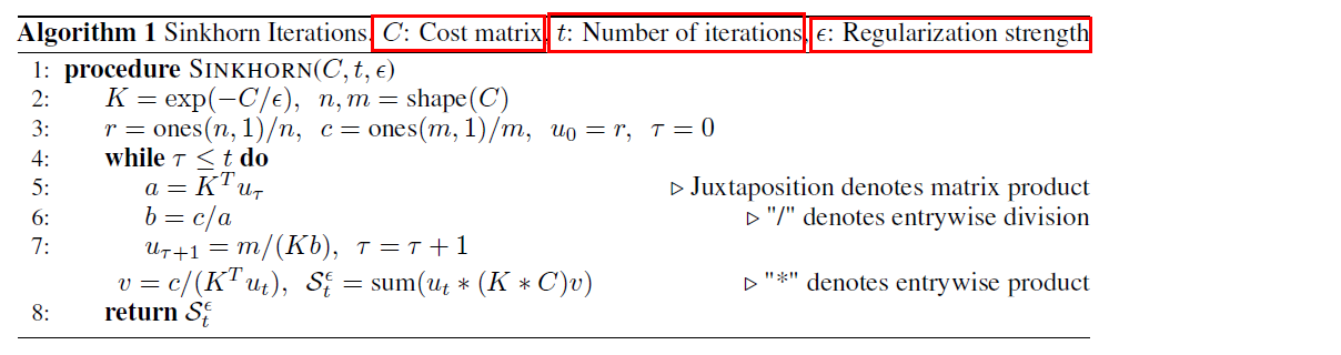
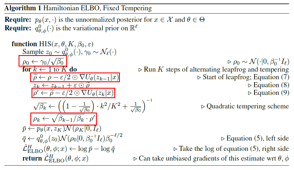
[ FULL PROCEDURE to get unbiased estimate of ELBO ]
\(\mathcal{L}_{\mathrm{ELBO}}(\theta, \phi ; x):=\int \log \hat{p}_{\theta}(x) q_{\theta, \phi}(u \mid x) d u \leq \log p_{\theta}(x)=: \mathcal{L}(\theta ; x)\) : ALGORITHM 1 (below)
-
\(\left(z_{0}, \rho_{0}\right)=\left(z_{0}, \gamma_{0} / \sqrt{\beta_{0}}\right)\).
for \(z_{0} \sim q_{\theta, \phi}^{0}(\cdot)\) and \(\gamma_{0} \sim \mathcal{N}\left(\cdot \mid 0, I_{\ell}\right) \equiv \mathcal{N}_{\ell}(\cdot)\).
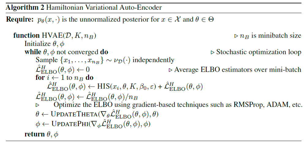
3. Stochastic Variational Inference
use above [Algorithm 1] within SVI!
Main interest : finding xxxxxx
Must use variational methods ( since the above can not be calculated exactly )
ELBO : xxxx
How to reduce the variance of ELBO?
-
in terms of expectations…. (Rao-Blackwellization)
\(\begin{aligned} \mathcal{L}_{\mathrm{ELBO}}^{H}(\theta, \phi ; x) &=\mathbf{E}_{\left(z_{0}, \rho_{0}\right) \sim q_{\theta, \phi}^{0}(\cdot, \cdot)}\left[\log \left(\frac{\bar{p}_{\theta}\left(x, z_{K}, \rho_{K}\right) \beta_{0}^{\ell / 2}}{q_{\theta, \phi}^{0}\left(z_{0}, \rho_{0}\right)}\right)\right] \\ &=\mathbf{E}_{z_{0} \sim q_{\theta, \phi}^{0}(\cdot), \gamma_{0} \sim \mathcal{N}_{\ell}(\cdot)}\left[\log p_{\theta}\left(x, z_{K}\right)-\frac{1}{2} \rho_{K}^{T} \rho_{K}-\log q_{\theta, \phi}^{0}\left(z_{0}\right)\right]+\frac{\ell}{2} \end{aligned}\).
- (under reparameterization) \(\left(z_{K}, \rho_{K}\right)=\mathcal{H}_{\theta, \phi}\left(z_{0}, \gamma_{0} / \sqrt{\beta_{0}}\right)\).
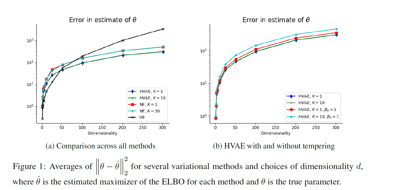
4. Experiments
4-1. Gaussian Model
Goal : learn model params
Model :
-
\(z \sim \mathcal{N}\left(0, I_{\ell}\right)\).
-
\(x_{i} \mid z \sim \mathcal{N}(z+\Delta, \mathbf{\Sigma}) \quad \text { independently }, \quad i \in[N]\).
( where \(\Sigma\) is constrained to be diagonal … \(\Sigma=\operatorname{diag}\left(\sigma_{1}^{2}, \ldots, \sigma_{d}^{2}\right)\) )
ELBO :
- \(\mathcal{L}_{\mathrm{ELBO}}(\theta, \phi ; \mathcal{D}):=\mathbf{E}_{z \sim q_{\theta, \phi}(\cdot \mid \mathcal{D})}\left[\log p_{\theta}(\mathcal{D}, z)-\log q_{\theta, \phi}(z \mid \mathcal{D})\right] \leq \log p_{\theta}(\mathcal{D})\).
Logarithm of unnormalized target :
- \(\log p_{\theta}(\mathcal{D}, z)=\sum_{i=1}^{N} \log \mathcal{N}\left(x_{i} \mid z+\Delta, \mathbf{\Sigma}\right)+\log \mathcal{N}\left(z \mid 0, I_{d}\right)\).
Use a HVAE with a variational prior, equal to the true prior ( = \(q^{0}=\mathcal{N}\left(0, I_{\ell}\right)\) ) and fixed tempering
Potential : \(U_{\theta}(z \mid \mathcal{D})=\log p_{\theta}(\mathcal{D}, z)\)
- its gradient : \(\nabla U_{\theta}(z \mid \mathcal{D})=z+N \boldsymbol{\Sigma}^{-1}(z+\Delta-x)\)
4-2. Generative Model for MNIST
using HVAE to improve convolutional VAE for binarized MNIST
Generative model
- \[z_{i} \sim \mathcal{N}\left(0, I_{\ell}\right)\]
- \[x_{i} \mid z_{i} \sim \prod_{j=1}^{d} \operatorname{Bernoulli}\left(\left(x_{i}\right)_{j} \mid \pi_{\theta}\left(z_{i}\right)_{j}\right)\]
Generative network ( decoder ) : \(\pi_{\theta}: \mathcal{Z} \rightarrow \mathcal{X}\)
Inference network ( encoder ) : \(q_{\theta, \phi}\left(z_{i} \mid x_{i}\right)=\mathcal{N}\left(z_{i} \mid \mu_{\phi}\left(x_{i}\right), \Sigma_{\phi}\left(x_{i}\right)\right)\)
- where \(\mu_{\phi}\) & \(\Sigma_{\phi}\) are separate outputs of the same NN
Apply HVAE on the top of the base convolutional VAE
5. Conclusion
-
Exploit Hamiltonian dynamics within SVi
-
Compared to previous methods..
- do not rely on learned reverse Markov kernels
- benefits from the use of tempering ideas
-
Use reparam trick to obtain unbiased estimators of gradients of ELBo
-
Can be interpreted as target-driven NFs
-
Jacobian computations required for ELBO are trivial
- Memory Cost could be large…