66.Variational Inference with Tail-Adaptive f-Divergence

Variational Inference with Tail-Adaptive f-Divergence (NeurIPS 2018)

Abstract

“VI with \(\alpha\) divergence”

• pros) mass-covering property
• cons) estimating & optimizing \(\alpha\) divergences require importance sampling, which may have large variance

Propose a new class of tail-adaptive f-divergences

• adaptively changes the convex function \(f\) with tail distn of the importance weights
• test this method on BNN

1. Introduction

success of VI depends on “proper divergence metric”

• (usually) KL-divergence \(KL(q \mid \mid p)\)

  ( but, this under-estimates the variance & miss important local modes of the true posterior )

• (alternative) f-divergence : \(D_{f}(p \mid \mid q)=\mathbb{E}_{x \sim q}\left[f\left(\frac{p(x)}{q(x)}\right)-f(1)\right]\)

  • \(f: \mathbb{R}_{+} \rightarrow \mathbb{R}\) : convex function
  • example) \(\alpha\)-divergence ( where \(f(t)=t^{\alpha} /(\alpha(\alpha-1))\) )

\(\alpha\)-divergence

• \(\alpha \rightarrow 0\) : KL-divergence \(KL(q \mid \mid p)\)
• \(\alpha \rightarrow 1\) : Reverse KL-divergence \(KL(p \mid \mid q)\)
  • ex) expectation propagation, importance weighted auto-encoder, cross entropy method
• \(\alpha=2\) : \(\chi^2\)-divergence

Why use \(\alpha\)-divergence? MASS COVERING property

• large values of \(\alpha\) :

  • pros) stronger mass-covering property

  • cons) high variance

    ( reason : involves estimating the \(\alpha\)-th power of density ratio \(\frac{p(x)}{q(x)}\))

• Thus, it is desirable to design an approach to choose \(\alpha\) adaptively and automatically, as \(q\) changes during the training iterations

  ( according to the distribution of the ratio \(\frac{p(x)}{q(x)}\))

Propose a new class of \(f\)-divergence which is tail-adaptive!

• uses different \(f\) according to the tail distn of density ratio \(\frac{p(x)}{q(x)}\)
• derive new adaptive \(f\)-divergence based VI
• Algorithm
  • replaces the \(f\) function with “rank-based function” of the empirical density ratio \(w=\frac{p(x)}{q(x)}\), at each gradient descent step of q

2. f-divergence and Friends

by minimizing the \(f\)-divergence between \(q_{\theta}\) and \(p\)

• \(\min _{\theta \in \Theta}\left\{D_{f}\left(p \mid \mid q_{\theta}\right)=\mathbb{E}_{x \sim q_{\theta}}\left[f\left(\frac{p(x)}{q_{\theta}(x)}\right)-f(1)\right],\right\}\).

• solve this by stochastic optimization

  ( by approximating the expectation \(\mathbb{E}_{x \sim q_{\theta}}[\cdot]\) using samples drawing from \(q_{\theta}\) at each iteration )

  
  

\(f\)-divergence

• ( by Jensen’s inequality ) \(\mathbb{D}_{f}(p \mid \mid q) \geq 0\) for any \(p\) and \(q .\)
• if \(f(t)\) is strictly convex at \(t=1,\) then \(D_{f}(p \mid \mid q)=0\) implies \(p=q\).

different \(f\)

• if \(f(t) = - \log t\) : (normal KL)
  • \(\mathrm{KL}(q \mid \mid p)=\mathbb{E}_{x \sim q}\left[\log \frac{q(x)}{p(x)}\right]\).
• if \(f(t) = t \log t\) : (reverse KL)
  • \(\mathrm{KL}(p \mid \mid q)=\mathbb{E}_{x \sim q}\left[\frac{p(x)}{q(x)} \log \frac{p(x)}{q(x)}\right]\).
• if \(f_{\alpha}(t)=t^{\alpha} /(\alpha(\alpha-1))\) & \(\alpha \in \mathbb{R} \backslash\{0,1\}\) : ( \(\alpha\) divergence )
  • \(D_{f_{\alpha}}(p \mid \mid q)=\frac{1}{\alpha(\alpha-1)} \mathbb{E}_{x \sim q}\left[\left(\frac{p(x)}{q(x)}\right)^{\alpha}-1\right]\).

\(\rightarrow\) \(\mathrm{KL}(q \mid \mid p)\) and \(\mathrm{KL}(p \mid \mid q)\) are the limits of \(D_{f_{\alpha}}(q \mid \mid p)\) when \(\alpha \rightarrow 0\) and \(\alpha \rightarrow 1\) respectively.

3. \(\alpha\)-divergence

Mass-covering property!

• reason : \(\alpha\)-divergence is proportional to the \(\alpha\)-th moment of density ratio \(p(x)/q(x)\)

  • large \(\alpha\) : large values of \(p(x)/q(x)\) will be penalized….. preventing \(p(x)>>q(x)\)

  • \(\alpha \leq 0\) : \(p(x)=0\) must imply \(q(x)=0\)…. to make \(D_{f_{\alpha}}(p \mid \mid q)\) finite

    • ex) \(\alpha=0\) : KL-divergence

Large \(\alpha\)

• stronger mass-covering properties
• also increase the variance

• desirable to keep \(\alpha\) large
• but ensure to keep \(\alpha\) smaller than \(\alpha_{*}\)

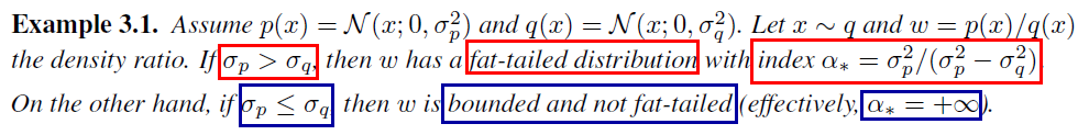
\(\rightarrow\) “estimate the tail index \(\alpha^{*}\) empirically at each iteration!”

4. Hessian-based Representation of \(f\)-Divergence

designing a generalization of \(f\)-divergence, in which \(f\) adaptively changes with \(p\) and \(q\)

• achieve strong mass-covering! ( equivalent to that of the \(\alpha\)-divergence with \(\alpha = \alpha^*\) )
• challenge of such adaptive \(f\)?
  • convex constraint over \(f\) is difficult to express computationally

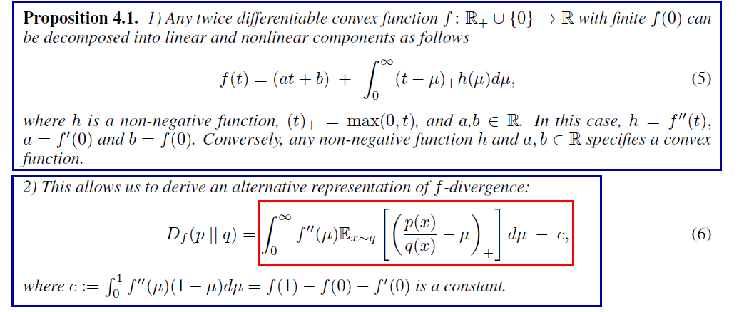
Specify a convex function \(f\) through \(f''\)

• this suggest that all \(f\)-divergences are conical combiations of a set of special \(f\)-divergences

  of form \(\mathbb{E}_{x \sim q}\left[(p(x) / q(x)-\mu)_{+}-f(1)\right] \text { with } f(t)=(t-\mu)_{+}\)

actually, we are more concerned in calculating the gradient ( rather than \(f\)-divergence itself )

\(\rightarrow\) gradients of \(\mathbb{D}_{f}\left(p \mid \mid q_{\theta}\right)\) is directly related to Hessian \(f''\)

Two ways of finding gradients

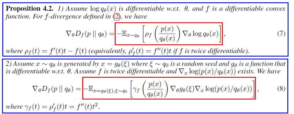
Gradient of \(f\)-divergence depends on \(f\) through \(\rho_f\) ( or \(\gamma_f\) )

• ex) \(\alpha\) divergence :
  • \[f(t)=t^{\alpha} /(\alpha(\alpha-1))\]
  • \[\rho_{f}(t)=t^{\alpha} / \alpha\]
  • \[\gamma_{f}(t)=t^{\alpha}\]
• ex) KL-divergence :
  • \[f(t)=-\log t\]
  • \[\rho_{f}(t)=\log t-1\]
  • \[\gamma_{f}(t)=1\]
• ex) Reverse KL-divergence :
  • \[f(t)=t \log t\]
  • \[\rho_{f}(t)=t\]
  • \[\gamma_{f}(t)=t\]

• eq (7) : score-function gradient

  • gradient free ( does not require calculating the gradient of \(p(x)\) )

• eq (8) : reparameterization gradient

  • gradient based ( involves \(\nabla_{x} \log p(x)\) )

  • has been shown that (8) is better than (7), because it leverages the gradient information \(\nabla_{x} \log p(x)\)

    & yields a lower variance estimator

5. Safe \(f\)-divergence with Inverse Tail Probability

It is sufficient to find an increasing function \(\rho_f\) ( or non-neg function \(\gamma_f\) ) to obtain adaptive \(f\)-divergence with computable gradients

To make \(f\)-divergence safe…..

• 1) need to find \(\rho_f\) or \(\gamma_f\) that adaptively depends on \(p\) and \(q\)
• 2) \(\mathbb{E}_{x \sim q}[\rho(p(x) / q(x))]<\infty\)
• 3) keep the function large ( to provide strong mode-covering property )

INVERSE of the tail probability achieves these 1)~3)!

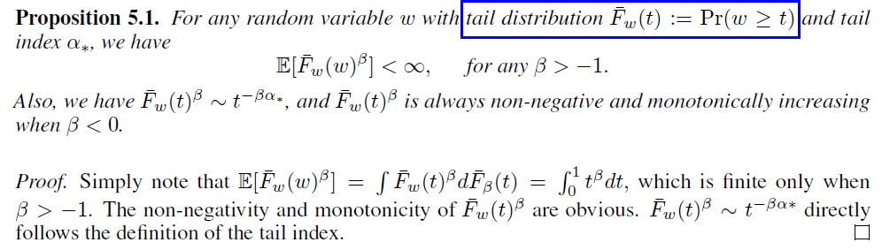
motivates to use “ \(\bar{F}_{w}(t)^{\beta}\) to define \(\rho_f\) ( or \(\gamma_f\) )”

• yields 2 versions of “safe” tail-adaptive \(f\)-divergence

6. Algorithm Summary

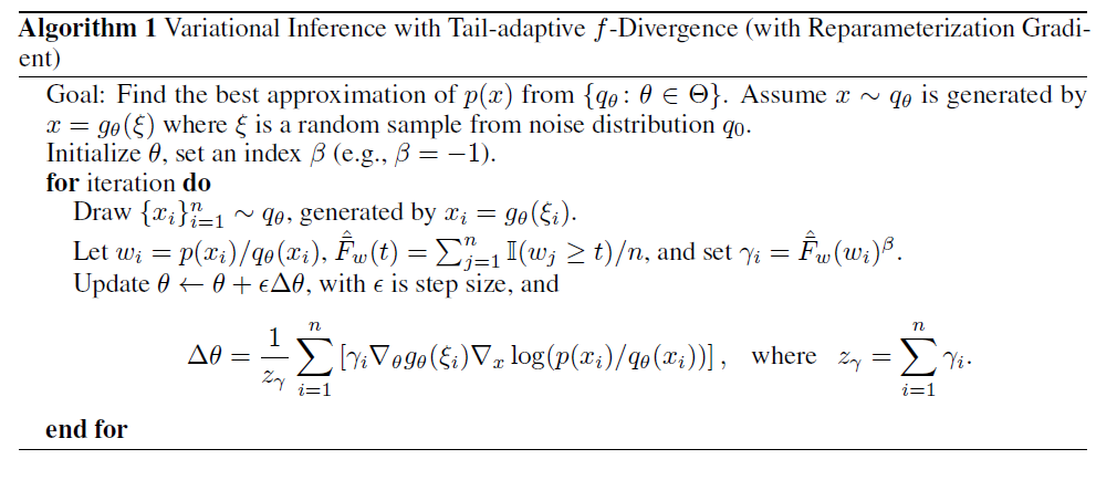
explicit form of \(\bar{F}_{w}(t)^{\beta}\) is unknown…. approximate it based on “empirical data” ( drawn from \(q\) )!

\(\rightarrow\) Let \(\left\{x_{i}\right\}\) be drawn from \(q\) and \(w_{i}=p\left(x_{i}\right) / q\left(x_{i}\right),\)

\(\rightarrow\) then we can approximate the tail probability with \(\hat{\bar{F}}_{w}(t)=\frac{1}{n} \sum_{i=1}^{n} \mathbb{I}\left(w_{i} \geq t\right) .\)

Compared with typical VI with reparameterized gradients….. this methods assings a

• WEIGHT \(\rho_{i}=\hat{F}_{w}\left(w_{i}\right)^{\beta}\)

  ( which is proportional \(\# w_{i}^{\beta}\), where \(\# w_{i}\) denotes the rank of data \(w_i\) )

• when taking \(-1<\beta<0\), this allows us to penalize places with high ratio \(p(x) / q(x)\), but avoid to be overly aggressive
• (in practice) use \(\beta=-1\)

7. Conclusion

present a new class of tail-adaptive \(f\)-divergence & exploit its application in VI & RL

compared to classic \(\alpha\)-divergence, our approach guarantees finite moments of density ratio & provides more stable importance weights & gradient estimates