81.Sparse Variational Inference ; Bayesian Coresets from Scrath

Sparse Variational Inference : Bayesian Coresets from Scrath (NeurIPS 2019)

Abstract

Recent work on Bayesian coresets :

• compressing the data, before inference algorithm!
• goal : both (1) scalability & (2) guaranteees on posterior approximation error

Proposition :

• formulate coreset construction as “sparsity-constrained VI within an exponential family”

1. Introduction

Bayesian Inference is typically intractable : use MCMC or VI

Both methods were created on per-model basis.

But developments in automated tools have made it accessible to practitioners

• ex) automatic differentiation, black-box gradient estimates, Hamiltonian transition kernels

• but that’s not enough! should be computationally scalable!

Bayesian Coreset ( = core of a dataset )

• alternative approach
• (assumption) large datasets = contain redundant data
• computationally inexpensive & simple

Proposition :

provide a new formulation of coreset construction as exponential family VI with sparsity constraint

2. Background

Pdf : \(\pi(\theta)\)

• decompose into \(N\) potentials : \(\left(f_{n}(\theta)\right)_{n=1}^{N}\)
• base density : \(\pi_{0}(\theta)\)

Decomposition : \(\pi(\theta):=\frac{1}{Z} \exp \left(\sum_{n=1}^{N} f_{n}(\theta)\right) \pi_{0}(\theta)\)

Often intractable to compute expectations under \(\pi\) exactly…

To reduce the cost of MCMC… instead run it on small, weighted subset of data = “Bayesian Coreset”

WEIGHT : (Sparse vector) \(w \in \mathbb{R}_{>0}^{N}\) ( only \(M \ll N\) are nonzero )

Approximate full log-density, with \(w\)-reweighted sum

• \(\pi_{w}(\theta):=\frac{1}{Z(w)} \exp \left(\sum_{n=1}^{N} w_{n} f_{n}(\theta)\right) \pi_{0}(\theta)\).,

  where only \(M \ll N,\) are nonzero ( \(\mid \mid w \mid \mid _{0}:=\sum_{n=1}^{N} \mathbb{1}\left[w_{n}>0\right] \leq M\) )

• \(\pi_{1}=\pi\) : full density

• If \(M \ll N,\) evaluating a function proportional to \(\pi_{w}\) is much less expensive than original \(\pi\)

• Goal : find a set of weights \(w\), that

  • 1) makes \(\pi_w\) as close as \(\pi\) ( for accuracy )
  • 2) maintain sparsity ( for speed )

into Sparse Regression Problem :

• \(\begin{array}{l} w^{\star}=\underset{w \in \mathbb{R}^{N}}{\arg \min } \mathbb{E}_{\hat{\pi}}\left[\left(\sum_{n=1}^{N} g_{n}-\sum_{n=1}^{N} w_{n} g_{n}\right)^{2}\right] \text { s.t. } w \geq 0, \mid \mid w \mid \mid _{0} \leq M \end{array}\).

  where \(g_{n}:=\left(f_{n}-\mathbb{E}_{\hat{\pi}}\left[f_{n}\right]\right)\)

  
  

using MC approximation :

• \(w^{\star}=\underset{w \in \mathbb{R}^{N}}{\arg \min } \mid \mid \sum_{n=1}^{N} \hat{g}_{n}-\sum_{n=1}^{N} w_{n} \hat{g}_{n} \mid \mid _{2}^{2} \text { s.t. } w \geq 0, \mid \mid w \mid \mid _{0} \leq M\).
• where
  • \(\left(\theta_{s}\right)_{s=1}^{S} \stackrel{\text { i.i.d. }}{\sim} \hat{\pi}\).
  • \(\hat{g}_{n}=\sqrt{S}^{-1}\left[g_{n}\left(\theta_{1}\right)-\bar{g}_{n}, \ldots, g_{n}\left(\theta_{S}\right)-\bar{g}_{n}\right]^{T} \in\).
• requires the selection of \(\hat{\pi}\)

3. Bayesian Coresets from scratch

new formulation of Bayesian coreset construction!

3-1. Sparse exponential family VI

treat as a sparse VI problem!

• \(w^{\star}=\underset{w \in \mathbb{R}^{N}}{\arg \min } \quad \mathrm{D}_{\mathrm{KL}}\left(\pi_{w} \mid \pi_{1}\right) \quad \text { s.t. } \quad w \geq 0,\mid \mid w \mid \mid _{0} \leq M\).
• \(\mathrm{D}_{\mathrm{KL}}\left(\pi_{w} \mid \pi_{1}\right)=\log Z(1)-\log Z(w)-\sum_{n=1}^{N}\left(1-w_{n}\right) \mathbb{E}_{w}\left[f_{n}(\theta)\right]\) ……… (a)

problem with (a) ?

• (1) \(Z(w)\) is unknown
• (2) computing the objective requires expectation under \(\pi_w\)

Propose New Algorithm!

• coresets from a sparse subset of an exponential family
• ( let \(f(\theta):=\left[\begin{array}{lll}f_{1}(\theta) \ldots f_{N}(\theta) \end{array}\right]^{T}\) )
• \(\pi_{w}(\theta):=\exp \left(w^{T} f(\theta)-\log Z(w)\right) \pi_{0}(\theta)\).
  • properties of exponential family : \(\mathbb{E}_{w}[f(\theta)]=\nabla_{w} \log Z(w)\). …….. (b)
• Using (b)…
  • before ) \(w^{\star}=\underset{w \in \mathbb{R}^{N}}{\arg \min } \quad \log Z(1)-\log Z(w)-\sum_{n=1}^{N}\left(1-w_{n}\right) \mathbb{E}_{w}\left[f_{n}(\theta)\right]\)
  • after ) \(w^{\star}=\underset{w \in \mathbb{R}^{N}}{\arg \min } \log Z(1)-\log Z(w)-(1-w)^{T} \nabla_{w} \log Z(w)\).

Derivative of objective function ( KL-div )

• \(\nabla_{w} \mathrm{D}_{\mathrm{KL}}\left(\pi_{w} \mid \pi_{1}\right)=-\nabla_{w}^{2} \log Z(w)(1-w)=-\operatorname{Cov}_{w}\left[f, f^{T}(1-w)\right]\).

• That is..

  • increase in \(w_n\) by small amount \(\rightarrow\) small decreases \(\mathrm{D}_{\mathrm{KL}}\left(\pi_{w} \mid \pi_{1}\right)\).

    ( by an amount proportional to the cov of the n\(^{th}\) potential \(f_{n}(\theta)\) with residual error \(\sum_{n=1}^{N} f_{n}(\theta)-\sum_{n=1}^{N} w_{n} f_{n}(\theta)\) under \(\pi_{w}\) )

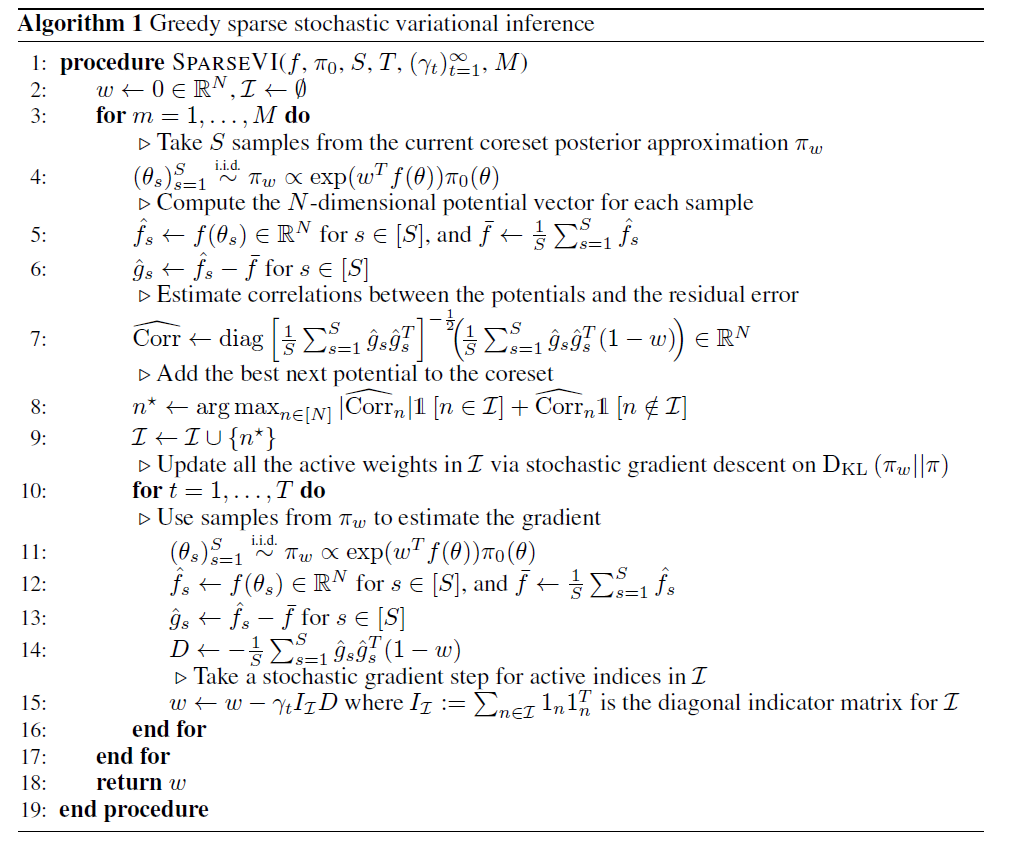
3-2. Greedy Selection

Naive approach : select potential that provides largest local decrease in KL-div

( = select the one with largest covariance with the residual error)

\(n^{\star}=\underset{n \in[N]}{\arg \max }\left\{\begin{array}{l} \left|\operatorname{Corr}_{w}\left[f_{n}, f^{T}(1-w)\right]\right| \quad w_{n}>0 \\ \operatorname{Corr}_{w}\left[f_{n}, f^{T}(1-w)\right] \quad \quad w_{n}=0 \end{array}\right.\).

use MC estimates via sampling from \(\pi_w\)

\(\widehat{\mathrm{Corr}}=\operatorname{diag}\left[\frac{1}{S} \sum_{s=1}^{S} \hat{g}_{s} \hat{g}_{s}^{T}\right]^{-\frac{1}{2}}\left(\frac{1}{S} \sum_{s=1}^{S} \hat{g}_{s} \hat{g}_{s}^{T}(1-w)\right) \quad \hat{g}_{s}:=\left[\begin{array}{c} f_{1}\left(\theta_{s}\right) \\ \vdots \\ f_{N}\left(\theta_{s}\right) \end{array}\right]-\frac{1}{S} \sum_{r=1}^{S}\left[\begin{array}{c} f_{1}\left(\theta_{r}\right) \\ \vdots \\ f_{N}\left(\theta_{r}\right) \end{array}\right]\).

3-3. Weight Update

after selecting new potential function \(n^{\star}\)…..

• add it to the active set of indicies \(\mathcal{I} \subseteq[N]\)

• Update the weights, by optimizing

  \(w^{\star}=\underset{v \in \mathbb{R}^{N}}{\arg \min } \mathrm{D}_{\mathrm{KL}}\left(\pi_{v} \mid \pi\right) \quad \text { s.t. } \quad v \geq 0, \quad\left(1-1_{\mathcal{I}}\right)^{T} v=0\).

• MC estimate (\(D\)) of gradient \(\nabla_{w} \mathrm{D}_{\mathrm{KL}}\left(\pi_{w} \mid \pi_{1}\right)\)

  \(D:=-\frac{1}{S} \sum_{s=1}^{S} \hat{g}_{s} \hat{g}_{s}^{T}(1-w) \in \mathbb{R}^{N}\).

Stochastic Gradient step : \(w_{n} \leftarrow w_{n}-\gamma_{t} D_{n}\).

Algorithm.

4. Conclusion

Exploit the fact that “coreset posteriors form an exponential family”

Introduce Sparse VI for Bayesian coreset construction!