82.Variational Denoising Network ; Toward Blind Noise Modeling and Removal

Variational Denoising Network : Toward Blind Noise Modeling and Removal ( NeurIPS 2019 )

Abstract

goal : Blind Image Denoising

method : new VI method

• integrates both (1) noise estimation & (2) image denoising into unique Bayesian framework

• approximate posterior : parameterized by DNN

• intrinsic clean image & noise variances as latent variables,

  conditioned on noisy input

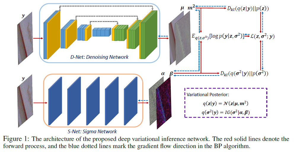
Variational Denoising Network ( VDN )

• perform denoising efficienctly due to its explicit form of posterior

1. Introduction

Image denoising?

• recover underlying clean image of noisy one

2 main methods

• (1) MAP ( with loss & regularized terms )
  • limitations due to assumption on image prior & noise
• (2) Deep Learning
  • first, collect large amount of “noisy-clean image pairs”
  • easy to overfit

Propose a new VI method!

• directly infer both (1) underlying clean image & (2) noise distn from a noisy image

2. Related Works

(1) model-driven MAP based

(2) data-driven Deep Learning based

Model-driven MAP based methods

• most classical image denoising methods
• fidelty/loss term & regularization
• pre-known image prior

Data-driven Deep Learning based Mtehods

• instead of pre-setting image prior, directly learn a denoiser
• input : large collection of noisy-clean image pair

3. Variational Denoising Network for Blind Noise Modeling

Training data \(D=\left\{\boldsymbol{y}_{j}, \boldsymbol{x}_{j}\right\}_{j=1}^{n}\).

• \(\boldsymbol{x}_{j}\) : clean image
• \(\boldsymbol{y}_{j}\) : noisy image

3-1. Constructing Full Bayesian Model based on training data

notation

• \(\boldsymbol{x}=\left[x_{1}, \cdots, x_{d}\right]^{T}\).
• \(\boldsymbol{y}=\left[y_{1}, \cdots, y_{d}\right]^{T}\).
• \(z \in \mathbb{R}^{d}\) :latent clean image

(1) generation process of noisy image :

• \(y_{i} \sim \mathcal{N}\left(y_{i} \mid z_{i}, \sigma_{i}^{2}\right), i=1,2, \cdots, d\).

(2) conjugate Gaussian prior on \(z\) :

• \(z_{i} \sim \mathcal{N}\left(z_{i} \mid x_{i}, \varepsilon_{0}^{2}\right), i=1,2, \cdots, d\).

(3) conjugate Inverse Gamma prior on \(\sigma^2\) :

• \(\sigma_{i}^{2} \sim \operatorname{IG}\left(\sigma_{i}^{2} \mid \frac{p^{2}}{2}-1, \frac{p^{2} \xi_{i}}{2}\right), i=1,2, \cdots, d\).

with (1) ~ (3) : full Bayesian model can be obtained.

Goal : Infer the posterior of latent variables \(z\) and \(\sigma^2\) from noisy image \(y\)

3-2. Variational Form of Posterior

Assume conditional independence between \(\sigma^2\) and \(z\)

\(q\left(\boldsymbol{z}, \boldsymbol{\sigma}^{2} \mid \boldsymbol{y}\right)=q(\boldsymbol{z} \mid \boldsymbol{y}) q\left(\boldsymbol{\sigma}^{2} \mid \boldsymbol{y}\right)\).

• \(q(\boldsymbol{z} \mid \boldsymbol{y})=\prod_{i}^{d} \mathcal{N}\left(z_{i} \mid \mu_{i}\left(\boldsymbol{y} ; W_{D}\right), m_{i}^{2}\left(\boldsymbol{y} ; W_{D}\right)\right)\).
• \(q\left(\boldsymbol{\sigma}^{2} \mid \boldsymbol{y}\right)=\prod_{i}^{d} \operatorname{IG}\left(\sigma_{i}^{2} \mid \alpha_{i}\left(\boldsymbol{y} ; W_{S}\right), \beta_{i}\left(\boldsymbol{y} ; W_{S}\right)\right)\).

where

• \(\mu_{i}\left(\boldsymbol{y} ; W_{D}\right)\) and \(m_{i}^{2}\left(\boldsymbol{y} ; W_{D}\right)\) : posterior params of latent variable \(z\) ….. D-Net (Denoising)
• \(\alpha_{i}\left(\boldsymbol{y} ; W_{S}\right)\) and \(\beta_{i}\left(\boldsymbol{y} ; W_{S}\right)\) : posterior params of \(\sigma^2\) ……. S-Net (Sigma)

3-3. Variational Lower Bound of Marginal Data Likelihood

Decompose its marginal likelihood

• \(\log p\left(\boldsymbol{y} ; \boldsymbol{z}, \boldsymbol{\sigma}^{2}\right)=\mathcal{L}\left(\boldsymbol{z}, \boldsymbol{\sigma}^{2} ; \boldsymbol{y}\right)+D_{K L}\left(q\left(\boldsymbol{z}, \boldsymbol{\sigma}^{2} \mid \boldsymbol{y}\right) \mid \mid p\left(\boldsymbol{z}, \boldsymbol{\sigma}^{2} \mid \boldsymbol{y}\right)\right)\).

  where \(\mathcal{L}\left(\boldsymbol{z}, \boldsymbol{\sigma}^{2} ; \boldsymbol{y}\right)=E_{q\left(\boldsymbol{z}, \boldsymbol{\sigma}^{2} \mid \boldsymbol{y}\right)}\left[\log p\left(\boldsymbol{y} \mid \boldsymbol{z}, \boldsymbol{\sigma}^{2}\right) p(\boldsymbol{z}) p\left(\boldsymbol{\sigma}^{2}\right)-\log q\left(\boldsymbol{z}, \boldsymbol{\sigma}^{2} \mid \boldsymbol{y}\right)\right]\) ( = ELBO )

• \(\log p\left(\boldsymbol{y} ; \boldsymbol{z}, \boldsymbol{\sigma}^{2}\right) \geq \mathcal{L}\left(\boldsymbol{z}, \boldsymbol{\sigma}^{2} ; \boldsymbol{y}\right)\).

Rewrite

• \(\mathcal{L}\left(\boldsymbol{z}, \boldsymbol{\sigma}^{2} ; \boldsymbol{y}\right)=E_{q\left(\boldsymbol{z}, \boldsymbol{\sigma}^{2} \mid \boldsymbol{y}\right)}\left[\log p\left(\boldsymbol{y} \mid \boldsymbol{z}, \boldsymbol{\sigma}^{2}\right)\right]-D_{K L}(q(\boldsymbol{z} \mid \boldsymbol{y}) \mid \mid p(\boldsymbol{z}))-D_{K L}\left(q\left(\boldsymbol{\sigma}^{2} \mid \boldsymbol{y}\right) \mid \mid p\left(\boldsymbol{\sigma}^{2}\right)\right)\).

• It can be integrated analytically!

• Term 1)

  \(E_{q\left(z, \sigma^{2} \mid y\right)}\left[\log p\left(\boldsymbol{y} \mid \boldsymbol{z}, \boldsymbol{\sigma}^{2}\right)\right]=\sum_{i=1}^{d}\left\{-\frac{1}{2} \log 2 \pi-\frac{1}{2}\left(\log \beta_{i}-\psi\left(\alpha_{i}\right)\right)-\frac{\alpha_{i}}{2 \beta_{i}}\left[\left(y_{i}-\mu_{i}\right)^{2}+m_{i}^{2}\right]\right\}\).

• Term 2)

  \(\begin{array}{c} D_{K L}(q(\boldsymbol{z} \mid \boldsymbol{y}) \mid \mid p(\boldsymbol{z}))=\sum_{i=1}^{d}\left\{\frac{\left(\mu_{i}-x_{i}\right)^{2}}{2 \varepsilon_{0}^{2}}+\frac{1}{2}\left[\frac{m_{i}^{2}}{\varepsilon_{0}^{2}}-\log \frac{m_{i}^{2}}{\varepsilon_{0}^{2}}-1\right]\right\} \end{array}\).

• Term 3)

  \(\begin{aligned} D_{K L}\left(q\left(\sigma^{2} \mid y\right) \mid \mid p\left(\sigma^{2}\right)\right)=\sum_{i=1}^{d}\left\{\left(\alpha_{i}\right.\right.&\left.-\frac{p^{2}}{2}+1\right) \psi\left(\alpha_{i}\right)+\left[\log \Gamma\left(\frac{p^{2}}{2}-1\right)-\log \Gamma\left(\alpha_{i}\right)\right] \\ &\left.+\left(\frac{p^{2}}{2}-1\right)\left(\log \beta_{i}-\log \frac{p^{2} \xi_{i}}{2}\right)+\alpha_{i}\left(\frac{p^{2} \xi_{i}}{2 \beta_{i}}-1\right)\right\} \end{aligned}\).

Final Objective Function : \(\min _{W_{D}, W_{S}}-\sum_{j=1}^{n} \mathcal{L}\left(z_{j}, \sigma_{j}^{2} ; y_{j}\right)\).

4. Conclusion

New Variational Inference Algorithm, called VDN(Variational Denoising Network) ,for blinding image denoising

Main Idea : learn an approximate posterior to the true posterior, with latent variables (clean image & noise variance)

proposed VDN is a generative method, which can estimate the noise distn from the input data.