
Sequential Monte Carlo
1. Motivation
Goal : “estimating unknown quantities”
Bayesian Models : 1) + 2)
- 1) prior distn for unknown quantities
- 2) likelihood functions
Often, observations arrive sequentially in time
\(\rightarrow\) interested in inference “on-line”
\(\therefore\) Update the posterior, as data become available
- key point? Computational Simplicity! ( not having to store all the data )
Examples )
-
Linear Gaussian state-space model : exact analytical expression
( this recursion is known as “Kalman Filter” )
-
Partially observed, finite state-space Markov chain
( known as “HMM filter” )
both rely on various assumptions….. but real world data is complex!
Sequential Monte Carlo
- simulation-based methods
- convenient to compute posterior
- very flexible & easy to implement, parallelisable
2. Problem Statement
Notation
-
observation : \(\left\{\mathbf{y}_{t} ; t \in \mathbb{N}^{*}\right\}\)
- unobserved signal : \(\left\{\mathbf{x}_{t} ; t \in \mathbb{N}\right\}, \mathbf{x}_{t} \in \mathcal{X}\)
- initial distribution : \(p\left(\mathbf{x}_{0}\right)\)
-
transition equation : \(p\left(\mathbf{x}_{t} \mid \mathbf{x}_{t-1}\right) .\)
- process : \(\left\{\mathrm{x}_{t} ; t \in \mathbb{N}\right\}\)
- marginal distribution : \(p\left(\mathbf{y}_{t} \mid \mathbf{x}_{t}\right)\)
Goal : “estimate recursively in time”…
- 1) posterior distribution : \(p\left(\mathbf{x}_{0: t} \mid \mathbf{y}_{1: t}\right),\)
- 2) its associated features ( ex. Marginal distribution \(p\left(\mathbf{x}_{t} \mid \mathbf{y}_{1: t}\right)\) )
- 3) expectations : \(I\left(f_{t}\right)=\mathbb{E}_{p\left(\mathbf{x}_{0: t} \mid \mathbf{y}_{1: t}\right)}\left[f_{t}\left(\mathbf{x}_{0: t}\right)\right] \triangleq \int f_{t}\left(\mathbf{x}_{0: t}\right) p\left(\mathbf{x}_{0: t} \mid \mathbf{y}_{1: t}\right) d \mathbf{x}_{0: t}\).
(1) Posterior distribution
- by Bayes theorem
- \(p\left(\mathbf{x}_{0: t} \mid \mathbf{y}_{1: t}\right)=\frac{p\left(\mathbf{y}_{1: t} \mid \mathbf{x}_{0: t}\right) p\left(\mathbf{x}_{0: t}\right)}{\int p\left(\mathbf{y}_{1: t} \mid \mathbf{x}_{0: t}\right) p\left(\mathbf{x}_{0: t}\right) d \mathbf{x}_{0: t}}\).
(2) Joint distribution ( + recursive formula )
- \(p\left(\mathbf{x}_{0: t+1} \mid \mathbf{y}_{1: t+1}\right)=p\left(\mathbf{x}_{0: t} \mid \mathbf{y}_{1: t}\right) \frac{p\left(\mathbf{y}_{t+1} \mid \mathbf{x}_{t+1}\right) p\left(\mathbf{x}_{t+1} \mid \mathbf{x}_{t}\right)}{p\left(\mathbf{y}_{t+1} \mid \mathbf{y}_{1: t}\right)}\).
(3) Marginal distribution
-
1) prediction
\(p\left(\mathbf{x}_{t} \mid \mathbf{y}_{1: t-1}\right)=\int p\left(\mathbf{x}_{t} \mid \mathbf{x}_{t-1}\right) p\left(\mathbf{x}_{t-1} \mid \mathbf{y}_{1: t-1}\right) d \mathbf{x}_{t-1}\).
-
2) Updating
\(p\left(\mathbf{x}_{t} \mid \mathbf{y}_{1: t}\right)=\frac{p\left(\mathbf{y}_{t} \mid \mathbf{x}_{t}\right) p\left(\mathbf{x}_{t} \mid \mathbf{y}_{1: t-1}\right)}{\int p\left(\mathbf{y}_{t} \mid \mathbf{x}_{t}\right) p\left(\mathbf{x}_{t} \mid \mathbf{y}_{1: t-1}\right) d \mathbf{x}_{t}}\).
3. Monte Carlo Methods
when one has large number of samples drawn from required posterior distn…
it is not difficult to approximate intractable integrals!
( but, sampling is HARD! )
Thus, need “alternative MC methods”, such as “Importance Sampling (IS)”
By making this recursive, one can obtain “Sequential Importance Sampling (SIS)”
3-1. Perfect MC sampling
simulate \(N\) independent samples ( particles ) \(\left\{\mathbf{x}_{0: t}^{(i)} ; i=1, \ldots, N\right\}\) , according to \(p\left(\mathbf{x}_{0: t} \mid \mathbf{y}_{1: t}\right)\)
Estimate of \(p\left(\mathbf{x}_{0: t} \mid \mathbf{y}_{1: t}\right)\) :
-
\(P_{N}\left(d \mathbf{x}_{0: t} \mid \mathbf{y}_{0: t}\right)=\frac{1}{N} \sum_{i=1}^{N} \delta_{\mathbf{x}_{0: t}^{(i)}}\left(d \mathbf{x}_{0: t}\right)\).
where \(\delta_{\mathbf{x}^{(i)}}\left(d \mathbf{x}_{0: t}\right)\) denotes the delta-Dirac mass located in \(\mathbf{x}_{0: t}^{(i)}\).
Following Estimate \(I\left(f_{t}\right)\) :
- \(I_{N}\left(f_{t}\right)=\int f_{t}\left(\mathrm{x}_{0: t}\right) P_{N}\left(d \mathrm{x}_{0: t} \mid \mathbf{y}_{1: t}\right)=\frac{1}{N} \sum_{i=1}^{N} f_{t}\left(\mathrm{x}_{0: t}^{(i)}\right)\).
By LLN…\(I_{N}\left(f_{t}\right) \underset{N \rightarrow+\infty}{\stackrel{a . s}{\longrightarrow}} I\left(f_{t}\right)\)
-
[proof]
\(\sigma_{f_{t}}^{2} \triangleq \mathbb{E}_{p\left(\mathbf{x}_{0: t} \mid \mathbf{y}_{1: t}\right)}\left[f_{t}^{2}\left(\mathbf{x}_{0: t}\right)\right]-I^{2}\left(f_{t}\right)<+\infty\).
thus, \(\operatorname{var}\left(I_{N}\left(f_{t}\right)\right)=\frac{\sigma_{f t}^{2}}{N}\)
-
if \(\sigma_{f_{t}}^{2}<+\infty,\)
\(\sqrt{N}\left[I_{N}\left(f_{t}\right)-I\left(f_{t}\right)\right] \underset{N \rightarrow+\infty}{\Longrightarrow} \mathcal{N}\left(0, \sigma_{f_{t}}^{2}\right)\).
BUT, it is usually impossible to sample EFFICIENTLY from \(p\left(\mathbf{x}_{0: t} \mid \mathbf{y}_{1: t}\right)\)
\(\therefore\) use MCMC! ( but MCMC are iterative algorithms, unsuited to recursive estimation problems )
Then..how?
3-2. Importance Sampling
Importance Sampling distribution
- ( = proposal distn, importance function )
- \(\pi\left(\mathbf{x}_{0: t} \mid \mathbf{y}_{1: t}\right)\).
\(I\left(f_{t}\right)=\frac{\int f_{t}\left(\mathbf{x}_{0: t}\right) w\left(\mathbf{x}_{0: t}\right) \pi\left(\mathbf{x}_{0: t} \mid \mathbf{y}_{1: t}\right) d \mathbf{x}_{0: t}}{\int w\left(\mathbf{x}_{0: t}\right) \pi\left(\mathbf{x}_{0: t} \mid \mathbf{y}_{1: t}\right) d \mathbf{x}_{0: t}}\).
- where importance weight : \(w\left(\mathbf{x}_{0: t}\right)=\frac{p\left(\mathbf{x}_{0: t} \mid \mathbf{y}_{1: t}\right)}{\pi\left(\mathbf{x}_{0: t} \mid \mathbf{y}_{1: t}\right)}\)
if we are able to simulate \(N\) particles …. according to “\(\pi\left(\mathbf{x}_{0: t} \mid \mathbf{y}_{1: t}\right)\)”,
\(\widehat{I}_{N}\left(f_{t}\right)=\frac{\frac{1}{N} \sum_{i=1}^{N} f_{t}\left(\mathbf{x}_{0: t}^{(i)}\right) w\left(\mathbf{x}_{0: t}^{(i)}\right)}{\frac{1}{N} \sum_{j=1}^{N} w\left(\mathbf{x}_{0: t}^{(i)}\right)}=\sum_{i=1}^{N} f_{t}\left(\mathbf{x}_{0: t}^{(i)}\right) \widetilde{w}_{t}^{(i)}\).
- where normalized importance weights are \(\widetilde{w}_{t}^{(i)}=\frac{w\left(\mathbf{x}_{0: t}^{(i)}\right)}{\sum_{j=1}^{N} w\left(\mathbf{x}_{0: t}^{(j)}\right)}\).
Therefore, posterior distribution approximation can become like…
- (using SAMPLING instead of INTEGRATION)
- \(\widehat{P}_{N}\left(d \mathbf{x}_{0: t} \mid \mathbf{y}_{1: t}\right)=\sum_{i=1}^{N} \widetilde{w}_{t}^{(i)} \delta_{\mathbf{x}_{0: t}^{(i)}}\left(d \mathbf{x}_{0: t}\right)\).
Conclusion
-
Importance Sampling = general MC integration method
-
but NOT ADEQUATE for recursive estimation
( one needs to get all \(y_{1:t}\) before estimating \(p(x_{0:t} \mid y_{1:t})\) )
( each time new data \(y_{t+1}\) comes in, need to recompute the importance weights over entire state )
3-3. Sequential Importance Sampling (SIS)
IS can be modified, so that…
- “no need to modify past simulated trajectories” \(\left\{\mathbf{x}_{0: t-1}^{(i)} ; i=1, \ldots, N\right\}\)
Importance function \(\pi\left(\mathbf{x}_{0: t} \mid \mathbf{y}_{1: t}\right)\) :
\(\begin{aligned}\pi\left(\mathbf{x}_{0: t} \mid \mathbf{y}_{1: t}\right)&=\pi\left(\mathbf{x}_{0: t-1} \mid \mathbf{y}_{1: t-1}\right) \pi\left(\mathbf{x}_{t} \mid \mathbf{x}_{0: t-1}, \mathbf{y}_{1: t}\right)\\&=\pi\left(\mathbf{x}_{0}\right) \prod_{k=1}^{t} \pi\left(\mathbf{x}_{k} \mid \mathbf{x}_{0: k-1}, \mathbf{y}_{1: k}\right)\end{aligned}\).
Importance function allows us to evaluate recursively!
- \(\widetilde{w}_{t}^{(i)} \propto \widetilde{w}_{t-1}^{(i)} \frac{p\left(\mathbf{y}_{t} \mid \mathbf{x}_{t}^{(i)}\right) p\left(\mathbf{x}_{t}^{(i)} \mid \mathbf{x}_{t-1}^{(i)}\right)}{\pi\left(\mathbf{x}_{t}^{(i)} \mid \mathbf{x}_{0: t-1}^{(i)}, \mathbf{y}_{1: t}\right)}\).
SOLUTION: adopt “prior distn” as “importance distn”
-
\(\pi\left(\mathbf{x}_{0: t} \mid \mathbf{y}_{1: t}\right)=p\left(\mathbf{x}_{0: t}\right)=p\left(\mathbf{x}_{0}\right) \prod_{k=1}^{t} p\left(\mathbf{x}_{k} \mid \mathbf{x}_{k-1}\right)\).
-
then, importance weight satisfies…
\(\widetilde{w}_{t}^{(i)} \propto \widetilde{w}_{t-1}^{(i)} p\left(\mathbf{y}_{t} \mid \mathbf{x}_{t}^{(i)}\right)\).
Conclusion
- SIS is an attractive…but just a constrained version of importance sampling
- inefficient in high-dimensional spaces
3-4. The Bootstrap Filter
as \(t\) increases… \(\tilde{w_t}^{(i)}\) becomes skewed…
to avoid this, need to introduce an additional selection step
Key Idea :
- 1) eliminate the particles having low importance weights \(\widetilde{w}_{t}^{(i)}\)
- 2) multiply particles having high importance weights
(before) \(\widehat{P}_{N}\left(d \mathbf{x}_{0: t} \mid \mathbf{y}_{1: t}\right)=\sum_{i=1}^{N} \widetilde{w}_{t}^{(i)} \delta_{\mathbf{x}_{0: t}^{(i)}}\left(d \mathbf{x}_{0: t}\right)\)
(after) \(P_{N}\left(d \mathbf{x}_{0: t} \mid \mathbf{y}_{1: t}\right)=\frac{1}{N} \sum_{i=1}^{N} N_{t}^{(i)} \delta_{\mathbf{x}_{0: t}^{(i)}}\left(d \mathbf{x}_{0: t}\right)\)
-
where \(N_{t}^{(i)}\) is the number of offspring associated to \(\mathbf{x}_{0: t}^{(i)}\)
( such that \(\sum_{i=1}^{N} N_{t}^{(i)}=N\) )
-
How to choose \(N_{t}^{(i)}\) ?
so that \(\int f_{t}\left(\mathbf{x}_{0: t}\right) P_{N}\left(d \mathbf{x}_{0: t} \mid \mathbf{y}_{1: t}\right) \approx \int f_{t}\left(\mathbf{x}_{0: t}\right) \widehat{P}_{N}\left(d \mathbf{x}_{0: t} \mid \mathbf{y}_{1: t}\right)\)
After selection step, surviving \(\mathbf{x}_{0: t}^{(i)},\) is the ones with \(N_{t}^{(i)}>0\)
Many ways to select \(N_{t}^{(i)}\)
-
ex) sampling \(N\) times from (discrete) distn \(\widehat{P}_{N}\left(d \mathbf{x}_{0: t} \mid \mathbf{y}_{1: t}\right)\)
( same as sampling \(N_{t}^{(i)}\) according to multinomial distn of params \(\tilde{w_t}^{(i)}\) )
Algorithm
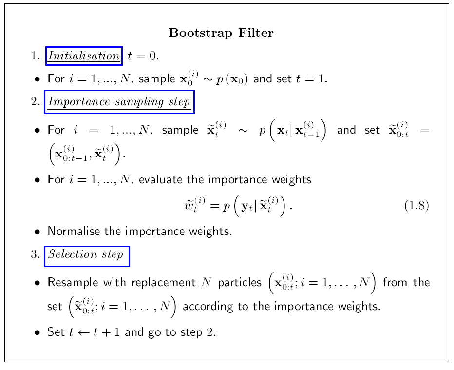
\(\widetilde{w}_{t}^{(i)}\) does not appear!
- because \(\mathbf{x}_{0: t-1}^{(i)}\) have uniform weights after resampling step at time \(t-1\)
Attractive Properties
-
1) quick & easy to implement
-
2) large extent modular
( = when changing the problem, only need to chance the expression for importance distn & weights )
-
3) able to be implemented in parallel computer