Neural Adaptive Sequential Monte Carlo
Abstract
SMC (Sequential Monte Carlo) = particle filtering
- sampling from an intractable target
- use sequence of simpler intermediate distn
- dependent on proposal distn
Presents a new method for “automatically adapting the proposal”,
using an approximation of KL-div between “true posterior” & “posterior distn”
\(\rightarrow\) Neural Adaptive SMC ( NASMC )
1. Introduction
SMC : the sequence constructs a proposal for importance sampling
Importance Sampling : dependent on the choice of proposal
- bad proposal \(\rightarrow\) low effective sample size & high variance
SMC have deeveloped approaches to solve this!
- ex) resampling to improve particle diversity, when the effective sample size is low
- ex) applying MCMC transition kernels
This paper suggests…“new gradient-based black-box adaptive SMC method”
- that automatically tunes flexible proposal distn
- can be assessed using KL-div between (1) target & (2) parameterized proposal
- very general & tractably handles complex proposal distn
2. Sequential Monte Carlo
2 fundamental SMC algorithms :
- **Sequential Importance Sampling (SIS) **
-
Sequential Importance Resampling (SIR)
-
probabilistic model containing hidden state (\(\boldsymbol{z}_{1: T}\)) & observed state(\(\boldsymbol{x}_{1: T}\))
\(\rightarrow\) joint distn : \(p\left(z_{1: T}, x_{1: T}\right)=p\left(z_{1}\right) p\left(x_{1} \mid z_{1}\right) \prod_{t=2}^{T} p\left(z_{t} \mid z_{1: t-1}\right) p\left(x_{t} \mid z_{1: t}, x_{1: t-1}\right)\)
(1) Sequential Importance Sampling (SIS)
Goal : approximate posterior, over hidden state sequence through a weighted set of \(N\) sampled trajectories drawn from simpler proposal distribution \(\left\{z_{1: T}^{(n)}\right\}_{n=1: N} \sim q\left(z_{1: T} \mid x_{1: T}\right)\)
- \(p\left(\boldsymbol{z}_{1: T} \mid \boldsymbol{x}_{1: T}\right) \approx \sum_{n=1}^{N} \tilde{w}_{t}^{(n)} \delta\left(\boldsymbol{z}_{1: T}-\boldsymbol{z}_{1: T}^{(n)}\right)\).
Factorize proposal distribution :
- \(q\left(\boldsymbol{z}_{1: T} \mid \boldsymbol{x}_{1: T}\right)=q\left(\boldsymbol{z}_{1} \mid \boldsymbol{x}_{1}\right) \prod_{t=2}^{T} q\left(\boldsymbol{z}_{t} \mid \boldsymbol{z}_{1: t-1}, \boldsymbol{x}_{1: t}\right)\).
Normalized Importance Weights ( defined by recursion )
- \(w\left(\boldsymbol{z}_{1: T}^{(n)}\right)=\frac{p\left(\boldsymbol{z}_{1: T}^{(n)}, \boldsymbol{x}_{1: T}\right)}{q\left(\boldsymbol{z}_{1: T}^{(n)} \mid \boldsymbol{x}_{1: T}\right)}\).
- \(\tilde{w}\left(\boldsymbol{z}_{1: T}^{(n)}\right)=\frac{w\left(\boldsymbol{z}_{1: T}^{(n)}\right)}{\sum_{n} w\left(\boldsymbol{z}_{1: T}^{(n)}\right)} \propto \tilde{w}\left(\boldsymbol{z}_{1: T-1}^{(n)}\right) \frac{p\left(\boldsymbol{z}_{T}^{(n)} \mid \boldsymbol{z}_{1: T-1}^{(n)}\right) p\left(\boldsymbol{x}_{T} \mid \boldsymbol{z}_{1: T}^{(n)}, \boldsymbol{x}_{1: T-1}\right)}{q\left(\boldsymbol{z}_{T}^{(n)} \mid \boldsymbol{z}_{1: T-1}^{(n)}, \boldsymbol{x}_{1: T}\right)}\).
Problem?
- highly skewed as \(t\) increases
\(\rightarrow\) use Sequential Importance Resampling (SIR)
(2) Sequential Importance Resampling (SIR)
-
add “additional step that resamples \(\boldsymbol{z}_{t}^{(n)}\) at time \(t\),
from a Multinomial distribution given by \(\tilde{w}\left(\boldsymbol{z}_{1: t}^{(n)}\right)\)
-
requires knowledge of full trajectory of previous samples
\(\rightarrow\) each new particle needs to update its ancestry information
( \(a_{\tau, t}^{(n)}\) : ancestral index of particle \(n\) at time \(t\) for state \(z_{\tau}\) )
2-1. The Critical Role of Proposal Distributions in SMC
Optimal choice : “intractable posterior” \(q_{\phi}\left(z_{1: T} \mid x_{1: T}\right)=p_{\theta}\left(z_{1: T} \mid x_{1: T}\right)\)
- ( factorization ) \(q\left(z_{t} \mid z_{1: t-1}, x_{1: t}\right)=p\left(z_{t} \mid z_{1: t-1}, x_{1: t}\right)\)
Bootstrap filter
- use prior as proposal distn!
- \(q\left(z_{t} \mid z_{1: t-1}, x_{1: t}\right)=p\left(z_{t} \mid z_{1: t-1}, x_{1: t-1}\right)\).
3. Adapting Proposals by Descending the Inclusive KL-divergence
“Proposal distn will be optimized using inclusive KL-div”
- \(\operatorname{KL}\left[p_{\theta}\left(\boldsymbol{z}_{1: T} \mid \boldsymbol{x}_{1: T}\right) \| q_{\phi}\left(\boldsymbol{z}_{1: T} \mid \boldsymbol{x}_{1: T}\right)\right]\).
Why this objective function?
-
1) direct measure of quality of the proposal
-
2) ( if true posterior lies in proposal family )
\(\rightarrow\) it has a global optimum at this point
-
3) ( if true posterior does not lie in proposal family )
\(\rightarrow\) tends to find proposal distn that have higher entropy than the original
-
4) derivative can be approximated efficiently
Gradient of negative KL-div ( + approximated using samples from SMC ) :
\(\begin{aligned}-\frac{\partial}{\partial \phi} \operatorname{KL}\left[p_{\theta}\left(z_{1: T} \mid \boldsymbol{x}_{1: T}\right) \| q_{\phi}\left(\boldsymbol{z}_{1: T} \mid \boldsymbol{x}_{1: T}\right)\right]&=\int p_{\theta}\left(\boldsymbol{z}_{1: T} \mid \boldsymbol{x}_{1: T}\right) \frac{\partial}{\partial \phi} \log q_{\phi}\left(\boldsymbol{z}_{1: T} \mid \boldsymbol{x}_{1: T}\right) d \boldsymbol{z}_{1: T}\\& \approx \sum_{t} \sum_{n} \tilde{w}_{t}^{(n)} \frac{\partial}{\partial \phi} \log q_{\phi}\left(\boldsymbol{z}_{t}^{(n)} \mid \boldsymbol{x}_{1: t}, \boldsymbol{z}_{1: t-1}^{A_{t-1}^{(n)}}\right) \end{aligned}\).
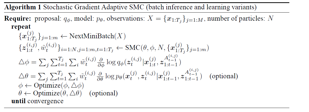
Online & Batch variants
- gradient update for the model params \(\theta\)
- \(\frac{\partial}{\partial \theta} \log \left[p_{\theta}\left(\boldsymbol{x}_{1: T}\right)\right] \approx \sum_{t} \sum_{n} \tilde{w}_{t}^{(n)} \frac{\partial}{\partial \theta} \log p_{\theta}\left(\boldsymbol{x}_{t}, \boldsymbol{z}_{t}^{(n)} \mid \boldsymbol{x}_{1: t-1}, \boldsymbol{z}_{1: t-1}^{A_{t-1}^{(n)}}\right)\).
Algorithm Summary