
Multiplicative Normalizing Flows for Variational Bayesian Neural Networks (2017)
Abstract
-
reinterpret “multiplicative noise” in NN as “auxiliary r.v” that augment the approximate posterior in VI for BNN
-
employ NF, while maintaining LRT & tractable ELBO
1. Introduction
cons of NN
- absence of enough data…overfit! ( ex. MRI data )
- NN trained with MLE or MAP : overconfident ( do not provide accurate CI )
\(\rightarrow\) thus, use Bayesian Inference ( point estimate (X), posterior (O) )
- ex) HMC, SGLD, Laplace approximation, EP, VI….
This paper adopts “Stochastic Gradient Variational Inference”
2. Multiplicative NF
2-1. VI & BNN
Reparameterization Trick
-
ELBO before) \(\begin{aligned} \mathcal{L}(\phi) &=\mathbb{E}_{q_{\phi}\left(\mathbf{W}_{1: L}\right)}\left[\log p\left(\mathbf{y} \mid \mathbf{x}, \mathbf{W}_{1: L}\right) +\log p\left(\mathbf{W}_{1: L}\right)-\log q_{\phi}\left(\mathbf{W}_{1: L}\right)\right] \end{aligned}\)
-
ELBO after) \(\begin{aligned} \mathcal{L} &=\mathbb{E}_{p(\epsilon)}[\log p(\mathbf{y} \mid \mathbf{x}, f(\phi, \epsilon))\left.+\log p(f(\phi, \epsilon))-\log q_{\phi}(f(\phi, \epsilon))\right] \end{aligned}\).
\(\rightarrow\) can be optimized with SGD
2-2. Improving the Variational Approximation
Mean Field, Mixture of delta peaks, matrix Gaussian that allow for nontrivial covariance among weights… \(\rightarrow\) limited!
2 famous methods
- 1) Normalizing Flow
- 2) Auxiliary Random variables ( ex. Dropout, Drop connect,….)
- introduce latent variables in the “posterior itself” !
How about applying NF to sample of the weight matrix from \(q(\mathbf{W})\)? EXPENSIVE!
( lose the benefit of LRT )
MNF (Multiplicative Normalizing Flow)
How to achieve both..
- 1) benefits of LRT
- 2) increase the flexibility with NF
\(\rightarrow\) rely on “auxiliary r.v” ( = multiplicative noise )….ex) Gaussian Dropout
-
\(\mathbf{z} \sim q_{\phi}(\mathbf{z}) ; \quad \mathbf{W} \sim q_{\phi}(\mathbf{W} \mid \mathbf{z})\).
\(q(\mathbf{W})=\int q(\mathbf{W} \mid \mathbf{z}) q(\mathbf{z}) d \mathbf{z}\).
-
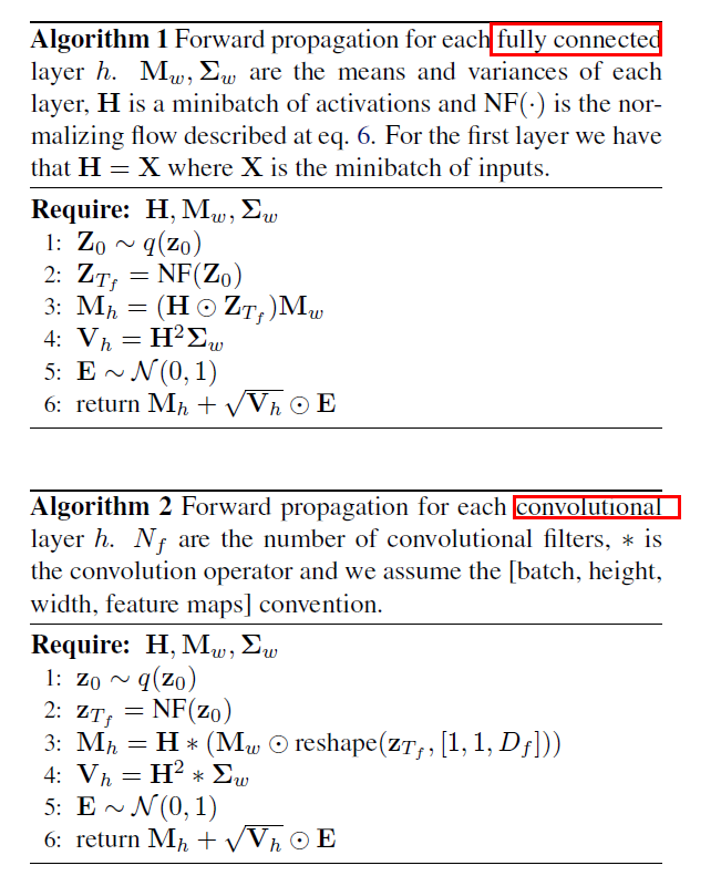
FC) \(q_{\phi}(\mathbf{W} \mid \mathbf{z})=\prod_{i=1}^{D_{i n}} \prod_{j=1}^{D_{o u t}} \mathcal{N}\left(z_{i} \mu_{i j}, \sigma_{i j}^{2}\right)\).
-
CNN) \(q_{\phi}(\mathbf{W} \mid \mathbf{z})=\prod_{i=1}^{D_{h}} \prod_{j=1}^{D_{w}} \prod_{k=1}^{D_{f}} \mathcal{N}\left(z_{k} \mu_{i j k}, \sigma_{i j k}^{2}\right)\).
By increasing the flexibility of mixing density \(q(\mathbf{z})\), …increase the flexibility of approximate posterior. ( \(\mathbf{z}\) is much lower dimension, compared to \(\mathbf{W}\) )
-
use masked RealNVP for NF
( using updates introduced in IAF )
\(\begin{array}{c} \mathbf{m} \sim \operatorname{Bern}(0.5) ; \quad \mathbf{h}=\tanh \left(f\left(\mathbf{m} \odot \mathbf{z}_{t}\right)\right) \\ \boldsymbol{\mu}=g(\mathbf{h}) ; \quad \boldsymbol{\sigma}=\sigma(k(\mathbf{h})) \\ \mathbf{z}_{t+1}=\mathbf{m} \odot \mathbf{z}_{t}+(1-\mathbf{m}) \odot\left(\mathbf{z}_{t} \odot \sigma+(1-\boldsymbol{\sigma}) \odot \boldsymbol{\mu}\right) \\ \qquad \log \mid \frac{\partial \mathbf{z}_{t+1}}{\partial \mathbf{z}_{t}} \mid =(1-\mathbf{m})^{T} \log \sigma \end{array}\).
2-3. Bounding the Entropy
\(q(\mathbf{W})=\int q(\mathbf{W} \mid \mathbf{z}) q(\mathbf{z}) d \mathbf{z}\). : no closed form!
Thus, entropy term \(-\mathbb{E}_{q(\mathbf{W})}[\log q(\mathbf{W})]\) is hard to calculate
\(\rightarrow\) introduce Lower Bound of entropy in terms of auxiliary distn \(r(\mathbf{z} \mid \mathbf{W})\).