93.Learning Deep Latent Gaussian Models with Markov Chain Monte Carlo

Learning Deep Latent Gaussian Models with Markov Chain Monte Carlo

Abstract

DLGM (Deep Latent Gaussian Models)

• powerful probabilistic model in high-dim data

• (mostly) use variational EM

This paper uses different approach…uses MCMC

1. Introduction

DLGM assumes that…

• 1) observed data were generated by sampling some latent variable
• 2) feeding them into DNN
• 3) add some noise

computational challenge : exact posterior is intractable

• (1) fit with VI! \(\rightarrow\) how to choose \(q\)?
• (2) use MCMC

This paper explore the advantages of MCMC !

By initializing chain with a sample from variational approximation… able to

• 1) speed up convergence
• 2) guarantee that posterior approximation is strictly better

2. Background

2-1. VAE & DLGMs

(1) DLGMs

Process

• step 1) Sample a vector \(z \in \mathbb{R}^{K}\) from \(N(0,1)\)

• step 2) Compute nonlinear function \(g_{\theta}(z)\)

  ( \(g\) is typically a DNN with param \(\theta\) )

• step 3) Sample \(x\) from some distribution \(f(g(z))\) that takes the output of \(g\) as a parameter.

Example

• \(g(z)=W \max \{0, V z+c\}+b\) ……. (1) output of one-hidden-layer ReLU network
• \(x_{d} \sim \mathcal{N}\left(g_{d}(z), \sigma\right)\). …………. (2) corrupted by Gaussian noise

Joint pdf : \(p(z, x)=\mathcal{N}(z ; 0, I) f\left(x ; g_{\theta}(z)\right)\).

Fit the model, maximizing the marginal likelihood!

\(\begin{aligned} \theta^{\star} &=\arg \max _{\theta} \frac{1}{N} \sum_{n} \log p_{\theta}\left(x_{n}\right) \\ &=\arg \max _{\theta} \frac{1}{N} \sum_{n} \log \int_{z} p_{\theta}\left(z, x_{n}\right) d z \end{aligned}\).

• but, integral over \(z\) is usually intractable!

Solution : variational EM

• maximize ELBO

  \(\begin{aligned} \mathcal{L}(\phi, \theta, x) & \triangleq \mathbb{E}_{q}\left[\log p_{\theta}(x \mid z)\right]-\mathrm{KL}\left(q_{z \mid x} \mid \mid p_{z}\right) \\ &=\log p_{\theta}(x)-\mathrm{KL}\left(q_{z \mid x} \mid \mid p_{z \mid x}\right) \leq \log p_{\theta}(x) \end{aligned}\).

Standard choice of DLGMs : choose \(q_{\phi}(z \mid x) \triangleq h\left(z ; r_{\phi}(x)\right)\)

• \(r_{\phi}(x)\) : output of an additional NN

• \(h(z ; r) :\) tractable distribution with parameters \(r\)

• common form of \(q\) : MVN

  ( mean field : \(q(z \mid x)=\prod_{k} q\left(z_{k} \mid x\right)\) )

• sometimes \(r\) is called “encoder” network & \(g\) is called “decoder” network

DLGM vs VAE

• DLGM : generative model
• VAE : paired encoder/decoder architecture for inference/generation

(2) VAEs

ELBO = \(\mathbb{E}_{q}\left[\log p_{\theta}(x \mid z)\right]-\mathrm{KL}\left(q_{z \mid x} \mid \mid p_{z}\right)\).

• \(\mathbb{E}_{q}\left[\log p_{\theta}(x \mid z)\right]\) is usually intractable

  \(\rightarrow\) estimate using MC sampling from \(q\)

  optimize ELBO, using stochastic optimization

2-2. Variational Pruning

skip

2-3. MCMC & HMC

MCMC’s advantage

• trade computation for accuracy without limit!

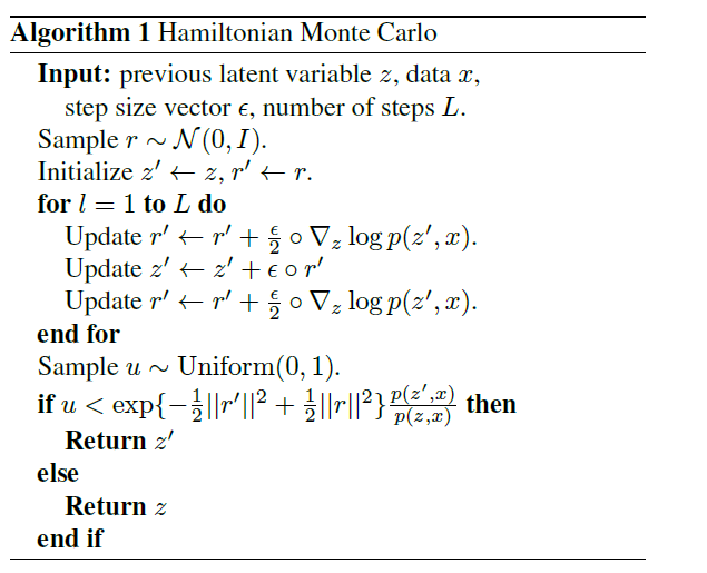
HMC (Hamiltonian MC, Hybrid MC)

• goal : sample from unnormalized distn ( \(p(z \mid x) \propto p(z, x)\) )

• augments this model to \(p(r, z \mid x) \triangleq \mathcal{N}(r ; 0, I) p(z \mid x)\)

  ( momentum variable \(r\) has the same dim as \(z\) )

• interpretation

  • latent variable \(z\) : position vector
  • \(\log p(z,x)\) : negative potential energy function
  • \(-\frac{1}{2} \mid \mid r \mid \mid ^{2}-\frac{D}{2} \log 2 \pi\) : negative kinetic energy function
  • Hamiltonian = potential + kinetic energy function

Algorithm

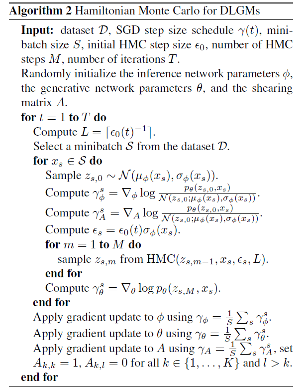
3. Practical MCMC for DLGMs

interested in optimizing “average marginal log-likelihood”

• \(\frac{1}{N} \sum_{n} \log p_{\theta}\left(x_{n}\right)=\frac{1}{N} \sum_{n} \log \int_{z} p_{\theta}\left(z, x_{n}\right) d z\).

gradient w.r.t \(\theta\) :

\(\begin{array}{l} \frac{1}{N} \sum_{n} \nabla_{\theta} \log \int_{z} p_{\theta}\left(z, x_{n}\right) d z \\ \quad=\frac{1}{N} \sum_{n} \int_{z} p_{\theta}\left(z \mid x_{n}\right) \nabla_{\theta} \log p_{\theta}\left(z, x_{n}\right) d z \end{array}\).

standard VAE

• approximates this expectation by replacing \(p(z \mid x)\) to a more tractable \(q(z \mid x)\)

• and computing MC estimate of \(\frac{1}{N} \sum_{n} \mathbb{E}_{q}\left[\nabla_{\theta} \log p\left(z, x_{n}\right)\right]\) :

  \(\gamma^{\mathrm{VAE}}=\frac{1}{\mid \mathcal{S} \mid } \sum_{s \in \mathcal{S}} \nabla_{\theta} \log p_{\theta}\left(z_{s}, x_{s}\right)\).

• but replacing above makes BIAS! how to solve…?

Naive approach : simply run HMC to estimate \(\nabla_{\theta} \log p(x)\)

• but… if not long enough… more BIAS!

\(\rightarrow\) instead, propose using HMC to improve on an INITIAL variational approximation

Core idea

• 1) Initialize HMC sampler ( with a sample from variational approximation )
• 2) run it for a small number of iterations
• 3) use the last sample to get estimate of \(\nabla_{\theta} \log p(x)\)

\(+\) define the refined distribution \(q'\)

\(q_{\epsilon, L, M}^{\prime}(z \mid x) \triangleq \int_{\tilde{z}} q(\tilde{z} \mid x) \operatorname{HMC}_{\epsilon, L, M}(z \mid \tilde{z}, x) d \tilde{z}\).

Regardless of how many HMC refinement steps we run, \(q^{\prime}\) is guaranteed to have lower KL divergence to the posterior \(p(z \mid x)\) than \(q\) does!

This observation suggests that we should care about making the initial variational distribution \(q(z \mid x)\) as close as possible to the posterior \(p(z \mid x)\)!

3-1. Refinements

2 refinements to the approach

(1) Learning a shared shearing matrix to rotate

DLGMs are unidentifiable up to a rotation

• \(p(z)=\mathcal{N}(z ; 0, I)\).

  \(g(z)=V \max \{0, W z+b\}+c\).

  \(p(x \mid z)=f(x ; g(z))\).

• \(p^{\prime}\left(z^{\prime}\right)=\mathcal{N}\left(z^{\prime} ; 0, I\right)\).

  \(g^{\prime}\left(z^{\prime}\right)=V \max \left\{0, W U z^{\prime}+b\right\}+c\).

  \(p^{\prime}\left(x \mid z^{\prime}\right)=f\left(x ; g\left(z^{\prime}\right)\right)\).

  ( where \(U\) is an arbitrary rotation matrix )

Result

• marginal distn of \(x\) : \(p(x)=p^{\prime}(x)\)

• marginal distn of \(z\) :\(g(z)=g^{\prime}\left(z^{\prime}\right)\)

• \(p(x \mid z)=p^{\prime}\left(x \mid z^{\prime}\right)\).

• BUT.. posterior : \(p(z \mid x)=p^{\prime}\left(U^{\top} z \mid x\right)\)

  ( This is bad, since MFVI is not rotationally invariant! performs best when no correlation! )

Solution : introduce extra lower triangular matrix \(A\) in generative network

( to correct for such rotations )

• model : \(z \sim \mathcal{N}(0, I) ; \quad z^{\prime} \triangleq A z ; \quad p(x \mid z) \triangleq f\left(g\left(z^{\prime}\right)\right)\)

• \(A\) : constrained to have diagonal = 1

  ( can not prune out any latent dim )

• If \(q(z \mid x)=\mathcal{N}\left(z ; \mu(x), \operatorname{diag}\left(\sigma(x)^{2}\right)\right)\)

  then \(q\left(z^{\prime} \mid x\right)=\mathcal{N}\left(z^{\prime} ; A \mu(x), \operatorname{Adiag}\left(\sigma(x)^{2}\right) A^{\top}\right)\)

(2) Setting per-variable step sizes and the number of leapfrog steps

Algorithm Summary