(paper) Manifold Mixup; Better Representations by Interpolating Hidden States

Manifold Mixup; Better Representations by Interpolating Hidden States

( https://arxiv.org/pdf/1806.05236.pdf )

Contents

1. Abstract
2. Introduction
3. Manifold Mixup
4. Manifold Mixup Flattens Representations

0. Abstract

DNN : excel at training data

\(\rightarrow\) not on slightly different test examples

( ex. distribution shifts, outliers, and adversarial examples )

propose Manifold Mixup

• a simple regularizer that encourages NN to predict less confidently on interpolations of hidden representations

• leverages semantic interpolations as additional training signal

  \(\rightarrow\) smoother decision boundaries at multiple levels of representation

• learn class-representations with fewer directions of variance.

1. Introduction

( hidden representations = \(z\) )

Troubling properties concerning \(z\) & decision boundaries of SOTA NN

1. decision boundary is often sharp and close to the data

2. vast majority of the \(z\) space corresponds to high confidence predictions

   ( both on and off of the data manifold )

propose Manifold Mixup (Section 2)

• a simple regularizer, by training NN on linear combinations of \(z\)

( Previous works ) Word embeddings : (e.g. king = man + woman   queen)

• shown that interpolations are an effective way of combining factors

High-level representations :

• often low-dimensional & useful to linear classifiers

  \(\rightarrow\) linear interpolations of \(z\) should explore meaningful regions of the feature space effectively

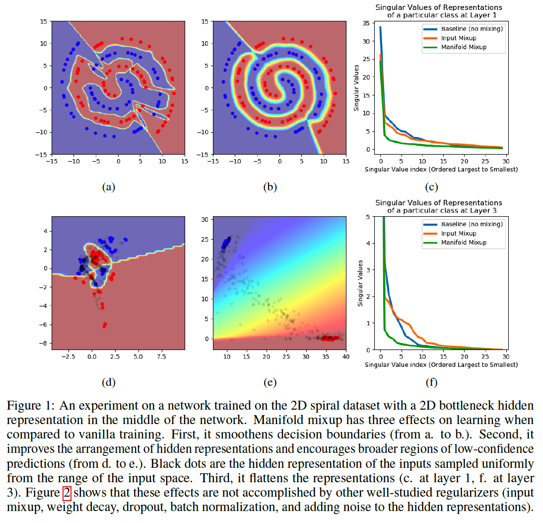
illustrates the impact of Manifold Mixup on a simple 2D classification task with small data.

vanilla DNN

• (Figure 1a) irregular decision boundary

• (Figure 1d) complex arrangement of \(z\)

• (Figure 1a & 1d) every point in raw & \(z\) space : very high confidence

DNN + Manifold Mixup

• (Figure 1b) smooth = decision boundary
• (Figure 1e) simpler (linear) arrangement of \(z\)

Summary

Two desirable properties of Manifold Mixup

1. the class-representations are flattened into a minimal amount of directions of variation
2. all points in-between these flat representations, most unobserved during training and off the data manifold, are assigned low-confidence predictions.

\(\rightarrow\) Manifold Mixup improves the hidden representations and decision boundaries of neural networks at multiple layers.

Why does Manifold Mixup improves generalization in DNN?

1. Leads to smoother decision boundaries at multiple levels of representation

   • ( = further away from the training data )
   • Smoothness and margin are well-established factors of generalization

2. Leverages interpolations in deeper hidden layers,

   • capture higher level information to provide additional training signal.

3. Flattens the class-representations

   • reduce their number of directions with significant variance

     ( = can be seen as a form of compression )

2. Manifold Mixup

Setting & Notation

• deep neural network \(f(x)=f_k\left(g_k(x)\right)\),
  • \(g_k\) : embedding function at layer \(k\)
  • \(f_k\) : mapping such \(z\) to the output \(f(x)\).

Training \(f\) using Manifold Mixup :

• step 1) select a random layer \(k\) from a set of eligible layers \(\mathcal{S}\) in the NN
  • ex) input layer \(g_0(x)\).
• step 2) process two random data minibatches \((x, y)\) and \(\left(x^{\prime}, y^{\prime}\right)\), until reaching layer \(k\).
  • ex) two intermediate minibatches \(\left(g_k(x), y\right)\) and \(\left(g_k\left(x^{\prime}\right), y^{\prime}\right)\).
• step 3) Input Mixup on these intermediate minibatches
  • ex) \(\left(\tilde{g}_k, \tilde{y}\right):=\left(\operatorname{Mix}_\lambda\left(g_k(x), g_k\left(x^{\prime}\right)\right), \operatorname{Mix}_\lambda\left(y, y^{\prime}\right)\right)\).
    • where \(\operatorname{Mix}_\lambda(a, b)=\lambda \cdot a+(1-\lambda) \cdot b\).
      • \(\left(y, y^{\prime}\right)\) : one-hot labels
      • \(\lambda \sim \operatorname{Beta}(\alpha, \alpha)\) : mixing coefficient
        • if \(\alpha=1.0\) \(\rightarrow\) equivalent to sampling \(\lambda \sim U(0,1)\).
• step 4) continue the forward pass using the mixed minibatch \(\left(\tilde{g}_k, \tilde{y}\right)\).
  • from layer \(k\) until the output
• step 5) output is used to compute the loss value

Mathematical Expression

minimize

\(L(f)=\underset{(x, y) \sim P}{\mathbb{E}} \underset{\left(x^{\prime}, y^{\prime}\right) \sim P}{\mathbb{E}} \underset{\lambda \sim \operatorname{Beta}(\alpha, \alpha)}{\mathbb{E}} \underset{k \sim \mathcal{S}}{\mathbb{E}} \ell\left(f_k\left(\operatorname{Mix}_\lambda\left(g_k(x), g_k\left(x^{\prime}\right)\right)\right), \operatorname{Mix}_\lambda\left(y, y^{\prime}\right)\right)\).

• when \(\mathcal{S}=\{0\}\), Manifold Mixup reduces to the original mixup

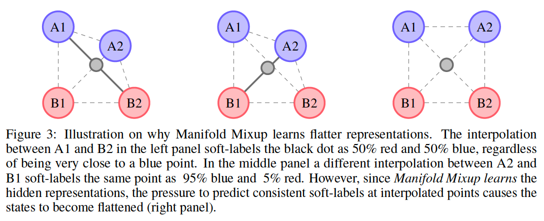
3. Manifold Mixup Flattens Representations

how Manifold Mixup impacts the \(z\)

( high level ) flattens the class-specific representations.

• reduces the number of directions with significant variance

  (akin to reducing their number of principal components)

(1) Theory

how the \(z\) are changed by Manifold Mixup

will show that if one performs mixup in a sufficiently deep hidden layer in a neural network,

\(\rightarrow\) then the loss can be driven to zero, if the dimensionality of that hidden layer \(\operatorname{dim}(\mathcal{H})\) is greater than the number of classes \(d\).

Notation

• \(\mathcal{X}\) : input space

• \(\mathcal{H}\) : representation space

• \(\mathcal{Y}\) : label space

• \(\mathcal{Z}=\mathcal{X} \times \mathcal{Y}\).

• set of functions realizable by NN

  • from the input to the representation : \(\mathcal{G} \subseteq \mathcal{H}^{\mathcal{X}}\)

  • from the representation to the output : \(\mathcal{F} \subseteq \mathcal{Y}^{\mathcal{H}}\)

\(J(P)=\inf _{g \in \mathcal{G}, f \in \mathcal{F}} \underset{(x, y),\left(x^{\prime}, y^{\prime}\right), \lambda}{\mathbb{E}} \ell\left(f\left(\operatorname{Mix}_\lambda\left(g(x), g\left(x^{\prime}\right)\right)\right), \operatorname{Mix}_\lambda\left(y, y^{\prime}\right)\right)\).

Notation

• \(P_D\) : empirical distribution defined by \(D=\left\{\left(x_i, y_i\right)\right\}_{i=1}^n\).
• \(f^{\star} \in \mathcal{F}\) and \(g^{\star} \in \mathcal{G}\) : minimizers of \(J(P)\) for \(P=P_D\).
• let \(\mathcal{G}=\mathcal{H}^{\mathcal{X}}, \mathcal{F}=\mathcal{Y}^{\mathcal{H}}\), and \(\mathcal{H}\) be a vector space.

\(\rightarrow\) mappings realizable by large NN are dense in the set of all continuous bounded functions

\(\rightarrow\) minimizer \(f^{\star}\) is a linear function from \(\mathcal{H}\) to \(\mathcal{Y}\).

Rewrite \(J(P)\) as …

\(J\left(P_D\right)=\inf _{h_1, \ldots, h_n \in \mathcal{H}} \frac{1}{n(n-1)} \sum_{i \neq j}^n\left\{\inf _{f \in \mathcal{F}} \int_0^1 \ell\left(f\left(\operatorname{Mix}_\lambda\left(h_i, h_j\right)\right), \operatorname{Mix}_\lambda\left(y_i, y_j\right)\right) p(\lambda) \mathrm{d} \lambda\right\}\).

• where \(h_i=g\left(x_i\right)\).

[ Theorem 1 ]

If \(\operatorname{dim}(\mathcal{H}) \geq d-1\) …

• (1) \(J\left(P_D\right)=0\)

• (2) corresponding minimizer \(f^{\star}\) is a linear function from \(\mathcal{H}\) to \(\mathbb{R}^d\).

Proof. the following statement is true if \(\operatorname{dim}(\mathcal{H}) \geq d-1\) :

\(\exists A, H \in \mathbb{R}^{\operatorname{dim}(\mathcal{H}) \times d}, b \in \mathbb{R}^d: A^{\top} H+b 1_d^{\top}=I_{d \times d}\).

• \(b 1_d^{\top}\) is a rank-one matrix
• rank of identity matrix is \(d\).

\(\rightarrow\) \(A^{\top} H\) only needs rank \(d-1\).

Let \(f^{\star}(h)=A^{\top} h+b\) for all \(h \in \mathcal{H}\).

Let \(g^{\star}\left(x_i\right)=H_{\zeta_i,:}\) be the \(\zeta_i\)-th column of \(H\), where \(\zeta_i \in\{1, \ldots, d\}\) stands for the class-index of the example \(x_i\).

These choices minimize \(J(P)\), since

\(\begin{align}&\ell\left(f^{\star}\left(\operatorname{Mix}_\lambda\left(g^{\star}\left(x_i\right), g^{\star}\left(x_j\right)\right)\right), \operatorname{Mix}_\lambda\left(y_i, y_j\right)\right) \\&= \ell\left(A^{\top} \operatorname{Mix}_\lambda\left(H_{\zeta_i,:}, H_{\zeta_j,:}\right)+b, \operatorname{Mix}_\lambda\left(y_{i, \zeta_i}, y_{j, \zeta_j}\right)\right)\\&=\ell(u, u) \\&=0 \end{align}\),

( the result follows from \(A^{\top} H_{\zeta_i,:}+b=y_{i, \zeta_i}\) for all \(i\). )

if \(\operatorname{dim}(\mathcal{H})>d-1\), then data points in \(\mathcal{H}\) have some degrees of freedom to move independently.

Corollary 1.

Consider the setting in Theorem 1 with \(\operatorname{dim}(\mathcal{H})>d-1\).

Let \(g^{\star} \in \mathcal{G}\) minimize \(J(P)\) under \(P=P_D\).

\(\rightarrow\) Then, the representations of the training points \(g^{\star}\left(x_i\right)\) fall on a \((\operatorname{dim}(\mathcal{H})-d+1)\) dim-subspace

Proof.

From the proof of Theorem \(1, A^{\top} H=I_{d \times d}-b 1_d^{\top}\).

The r.h.s. of this expression is a rank\((d-1)\) matrix for a properly chosen \(b\).

Thus, \(A\) can have a null-space of \(\operatorname{dimension} \operatorname{dim}(\mathcal{H})-d+1\).

This way, one can assign \(g^{\star}\left(x_i\right)=H_{\zeta_i,:}+e_i\),

• where \(H_{\zeta_i,:}\) is defined as in the proof of Theorem 1
• where \(e_i\) are arbitrary vectors in the null-space of \(A\), for all \(i=1, \ldots, n\).

Summary

implies that if the Manifold Mixup loss is minimized

\(\rightarrow\) then the representation of each class lies on a subspace of dimension \(\operatorname{dim}(\mathcal{H})-d+1\).

In the extreme case where …

(1) \(\operatorname{dim}(\mathcal{H})=d-1\),

• each class representation will collapse to a single point

  ( = meaning that \(z\) would not change in any direction, for each class-conditional manifold )

(2) general case with larger \(\operatorname{dim}(\mathcal{H})\)

• the majority of directions in \(\mathcal{H}\)-space will be empty in the class-conditional manifold.