(paper) Contrastive Masked Autoencoders are Stronger Vision Learners

Contrastive Masked Autoencoders are Strong Vision Learners

( https://arxiv.org/pdf/2207.13532.pdf )

Contents

1. Abstract
2. Introduction
3. Related Works
4. Method
   1. Framework
   2. View Augmentations
   3. Training Objective

0. Abstract

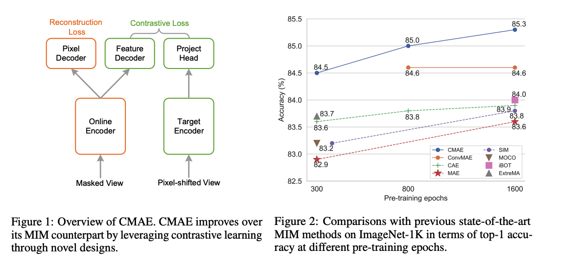
propose Contrastive Masked Autoencoders (CMAE)

• CL + MIM : leverages their respective advantages
• learns representations with both strong
  • (1) instance discriminability
  • (2) local perceptibility.
• consists of two branches
  • (1) online branch : asymmetric encoder-decoder
  • (2) target branch : momentum updated encoder

Training procedure

• online encoder : reconstructs original images from latent representations of masked images
• target encoder : fed with the full images
  • enhances the feature discriminability via CL with its online counterpart

To make CL compatible with MIM…

\(\rightarrow\) introduce two new components

• (1) pixel shifting ( for generating plausible positive views )

• (20 feature decoder ( for complementing features of contrastive pairs )

Summary

• effectively improves the representation quality
• transfer performance over its MIM counterpart

1. Introduction

Masked image modeling (MIM)

• increasing attention recently in SSL
  • due to its method simplicity & capability of learning rich and holistic representations
• procedure
  • step 1) randomly mask a large portion of the training image patches
  • step 2) use an AE to reconstruct masked patches

MIM vs CL

• CL : naturally endow the pretained model with strong instance discriminability.

• MIM : focuses more on learning local relations in input image for fulfilling the reconstruction

  \(\rightarrow\) suspected that MIM is less efficient in learning discriminative representations.

Can we leverage CL to further strengthen the representation learned by MIM methods?

• few contemporary works attempt to train vision representation models by simply combining CL + MIM objectives

  \(\rightarrow\) only show marginal performance gain

• it is non-trivial to fully leverage the advantages of both CL & MIM

This paper : aim to explore a possible way to boost the MIM with CL

\(\rightarrow\) findings : input view augmentation and latent feature alignment play important roles

contrastive MAE (CMAE)

• adopts a siamese architecture

  • online branch :

    • online updated asymmetric encoder-decoder

    • learns latent representations to reconstruct masked images from a few visible patches

      ( inputs only contain the visible patches )

  • target branch :

    • a momentum encoder that provides contrastive learning supervision

      ( fed with the full set of image patches )

• To leverage CL, introduce an auxiliary feature decoder into the online branch

  • output featuers : used for CL with the momentum encoder outputs.

• 2 decoders

  • (1) Pixel Decoder : predict the image pixel and perform the MIM task
  • (2) Feature Decoder : recover the features of masked tokens. Since the semantics of each patch are incomplete and ambiguous, it is

2. Related Works

MIM

Based on the reconstruction target … these methods can be devided into:

• (1) pixel-domain reconstruction
• (2) auxiliary features/tokens prediction

SIM & MAE

• propose to reconstruct the raw pixel values …

  • (SimMIM) from the full set of image patches
  • (MAE) from partially observed patches

  to reconstruct the raw image.

• SimMIM vs MAE : MAE is more pre-training efficient

  ( \(\because\) masking out a large portion of input patches. )

etc

• MaskFeat : introduces the low-level local features as the reconstruction target

• CIM : opts for more complex input.

Several methods adopt an extra model to generate the target

• BEiT : uses the discretized tokens from an offline tokenizer
• PeCo : uses an offline visual vocabulary to guide the encoder
• CAE : uses both the online target and offline network to guide the training of encoder
• iBOT : introduces an online tokenizer to produce the target to distill the encoder
• SIM : adopts the siamese network
• MSN : matches the representation of masked image to that of original image using a set of learnable prototypes.

(common) focus on learning relations among the tokens in the input image

• instead of modeling the relation among different images as CL

\(\rightarrow\) less discriminative

3. Method

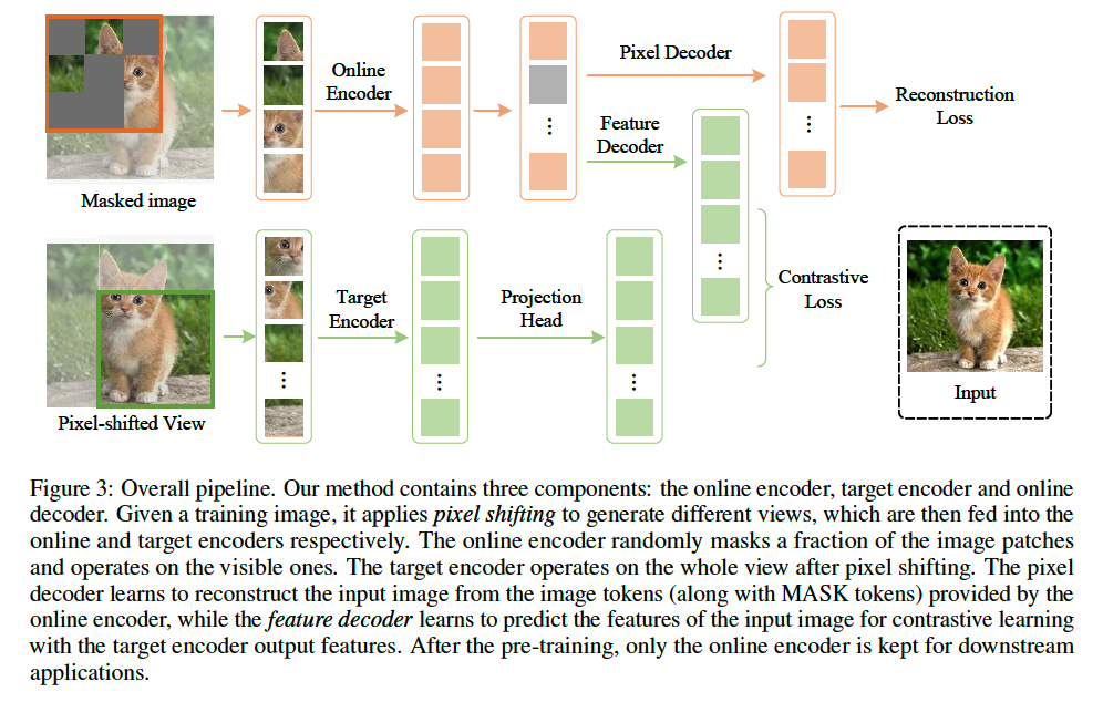
(1) Framework

Notation

input image \(I_s\)

• fed into ENCODER :
  • tokenized into a token sequence \(\left\{x_i^s\right\}_{i=1}^N\)
    • \(N\) : number of image patches (tokens)
    • denote the visible tokens as \(\left\{x^v\right\}\).
• fed into DECODER :
  • denoted as \(\left\{x_j^t\right\}_{j=1}^N\)

a) Online encoder \(\mathcal{F}_s\)

( adopts Vision Transformer (ViT) architecture )

1. Input : token sequence \(\left\{x_i^s\right\}_{i=1}^N\),

2. Masking : mask out a large ratio of patches

3. Feed unmasked images

   • maps the visible tokens \(x_s^v\) to embedding features \(z_s^v\).

Procedure

• step 1) embeds the visible tokens \(x_s^v\) by linear projection as token embeddings

• step 2) adds the positional embeddings \(p_s^v\).

• step 3) feed the fused embedding to a sequence of transformer blocks

  \(\rightarrow\) get the embedding features \(z_s^v\).

  \(z_s^v=\mathcal{F}_s\left(x_s^v+p_s^v\right)\).

• step 4) (After pre-training) use online encoder \(\mathcal{F}_s\) to extracting image representations

b) Target Encoder \(\mathcal{F}_t\)

to provide contrastive supervision for the online encoder

• to learn discriminative representations
• only serves for contrastive learning

Architecture : same as \(\mathcal{F}_s\)

• but takes the whole image as input ( no masking )
  • to reserve the semantic integrity

Unlike tokens in NLP, whose semantic are almost certain, image token is ambiguous in its semantic meaning

\(\rightarrow\) adopt global representations for CL

\(\rightarrow\) mean-pooled feature of target encoder is used for its simplicity

• \(z_t=\frac{1}{N} \sum_{j=1}^N \mathcal{F}_t\left(x_j^t\right)\).
  • \(x_j^t\) : input token for target encoder
  • \(z_t\) : representation of the input image

Update

• update parameters of the target encoder by EMA
• \(\theta_t \leftarrow \mu \theta_t+(1-\mu) \theta_s\).
  • \(\mu\) : fixed as 0.996
• ( Momentum update is used, since it stabilizes the training by fostering smooth feature changes, as found in MoCo & BYOL )

c) Online Decoder

• Input : receives both the encoded visible tokens \(z_s^v\) and MASK tokens \(z_s^m\).

• Goal : map the ( latent features \(z_s^v\) & MASK token features ) to the feature space of the target encoder and the original images

• Position embeddings : added to input tokens.

• 2 branches of decoder structure

  • (1) pixel decoder \(\mathcal{G}_p\)

    • learns to reconstruct the pixel of the masked patches
    • use the full set of tokens ( = both \(z_s^v\) and \(z_s^m\) ) to predict the pixel of patches \(y^m\).
    • learn holistic representation for each patch in an image
    • stacked transformer blocks : \(y_m^{\prime}=\mathbb{I} \cdot \mathcal{G}_p\left(z_s^v, z_s^m\right)\)
      • \(\mathbb{I}\) : select only masked tokens
      • \(y_m\) : output of masked tokens
      • \(y_m\) : output prediction ~

  • (2) feature decoder \(\mathcal{G}_f\)

    • recover the feature of masked tokens.

    • same structure as \(\mathcal{G}_p\)

      • but non-shared parameters for serving a different learning target

    • given the encoded visible tokens \(z_s^v\), & masked tokens \(z_s^m\) …

      \(\rightarrow\) predict the feature of masked tokens.

    • Mean pooling

      • on the output of feature decoder as the whole image representation \(y_s\)
      • \(y_s=\frac{1}{N} \sum \mathcal{G}_f\left(z_s^v, z_s^m\right)\).

(2) View augmentations

( In general )

• MIM : only utilizes 1 view of the input image

• CL : adopts 2 augmented views.

To make MIM and CL be compatible with each other..

\(\rightarrow\) generates two different views & feeds them to its online and target branches, respectively

(3) Training Objective

a) Reconstruction Loss

• use the normalized pixel as target
• loss : MSE
• loss only on masked patches
• \(L_r=\frac{1}{N_m} \sum\left(y_m^{\prime}-y_m\right)^2\).

b) Contrastive Loss

describe the contrastive loss design of our method from 2 aspects:

• (1) loss function
• (2) head structure

[ loss function ]

2 widely used styles

• (1) InfoNCE loss
  • seeks to simultaneously pull close positive views from the same sample and push away negative samples
• (2) BYOL-style loss.
  • only maximizes the similarity between positive views

Aanalyze them separately due to their diverse effects on representation learning.

\(\rightarrow\) observe better performance using InfoNCE

[ head structure ]

adopt the widely used “projection prediction”

append the …

• “projection-prediction” head to feature decoder

• “projection” head to target encoder

  • also updated by EMA

Due to the large differences on generating inputs for online/target encoder ..

\(\rightarrow\) use asymmetric contrastive loss

Procedure

• output of feature decoder \(y_s\) :
  • transformed by the “projection-prediction” structure to get \(y_s^p\).
• output of target encoder \(z_t\) :
  • apply the projection head to get \(z_t^p\).

Cosine similarity \(\rho\) : \(\rho=\frac{y_s^p \cdot z_t^p}{ \mid \mid y_s^p \mid \mid _2 \mid \mid z_t^p \mid \mid _2}\)

• \(\rho^{+}\) : positive pairs cosine similarity
  • When \(y_s^p\) and \(z_t^p\) are from the same image
• . \(\rho_j^{-}\) :cosine similarity for the \(j\)-th negative pair.

( use the \(z_t^p\) from different images in a batch to construct negative pairs )

Loss function of InfoNCE loss :

• \(L_c=-\log \frac{\exp \left(\rho^{+} / \tau\right)}{\exp \left(\rho^{+} / \tau\right)+\sum_{j=1}^{K-1}\left(\exp \left(\rho_j^{-} / \tau\right)\right)}\).

Final Loss

\(L=L_r+\lambda_c L_c\).