[continual] (paper 5) Gradient Episodic Memory for Continual Learning

Gradient Episodic Memory for Continual Learning

Contents

1. Abstract
2. Introduction
3. A Framework for Continual Learning
4. Gradient of Epsiodic Memory (GEM)
5. Algorithm

0. Abstract

2가지를 제안함

• (1) metrics to evaluate models learning over a continuum of data
• (2) model for continual learning, called GEM (Gradient Episodic Memory)

1. Introduction

(대부분의) Supervise learning의 특징

• input data에 대한 i.i.d 가정
• 목표 : 보지 못한 데이터 (unseen data)에 대한 loss를 minimize하도록 학습됨
• ERM (Empirical Risk Minimization) principle 차용

하지만, 인간들은 다르다.

• Humans observe data as an ORDERED SEQUENCE! ( i.i.d가 아니다 )
• 적은 수의 데이터 밖에 기억하지 못한다

\(\therefore\), 현실적으로, ERM을 적용하면 catastrophic forgetting 발생한다!

\(\rightarrow\) 이 paper의 목표 : ERM과 human-like learning 사이의 gap 줄이기!

Notation

continuum of data : \(\left(x_{1}, t_{1}, y_{1}\right), \ldots,\left(x_{i}, t_{i}, y_{i}\right), \ldots,\left(x_{n}, t_{n}, y_{n}\right)\)

• 이들은 서로 i.i.d가 아니다
• task descriptor : \(t_{i} \in \mathcal{T}\)
• data pair : \(\left(x_{i}, y_{i}\right) \sim P_{t_{i}}\)

challenges unknown to ERM

• 1) Non-iid input data

• 2) Catastrophic forgetting

• 3) Transfer learning

  ( 만약 continuum내의 task들이 서로 related 되어있다면, transfer learninng을 활용할 여지 O )

2. A Framework for Continual Learning

( 가정 : continuum들은 locally i.i.d이다. 즉, \(\left(x_{i}, y_{i}\right) \stackrel{i i d}{\sim} P_{t_{i}}(X, Y)\) )

Training Protocol & Evaluation Metrics

일반적으로, sequence of tasks에 대해 학습하는 것은, 아래와 같은 setting을 가진다.

• 1) task의 수는 적다
• 2) task 별 데이터 수는 충분하다
• 3) 각 task내의 example에 대해 여러번의 pass를 거침
• 4) average performance across all tasks를 metric으로 삼음

하지만, 이 논문은 보다 “human-like” setting을 가정한다 ( 보다 현실적 )

그러기 위해….

• training time에 learner에게 ONLY ONE example at a time만을 제공!

• 똑같은 data가 2번 제공되지 않음

• tasks는 sequence로 들어옴

• 아래의 (1) 뿐만 아니라, (2) 또한 중시함

  • (1) performance across tasks

  • (2) ability of learner to TRANSFER KNOWLEDGE

    ( 아래의 2가지 measure 참고 )

측정하고자 하는 measure

1. Backward Transfer (BWT)
   • task \(t\)에 대해서 학습하는 것이 PREVIOUS task \(t-1,...1\)에 미치는 영향
   • positive BWT & negative BWT ( = catastrophic forgetting )
2. Forward Transfer (FWT)
   • task \(t\)에 대해서 학습하는 것이 FUTURE task \(t+1,...N\)에 미치는 영향
3. Test classsification accuracy : \(R_{i,j}\)
   • task \(t_i\)를 관측한 뒤, task \(t_j\)에 대한 accuarcy

제안한 3가지 metric

\(\begin{aligned} \text { Average Accuracy: } \mathrm{ACC} &=\frac{1}{T} \sum_{i=1}^{T} R_{T, i} \\ \text { Backward Transfer: } \mathrm{BWT} &=\frac{1}{T-1} \sum_{i=1}^{T-1} R_{T, i}-R_{i, i} \\ \text { Forward Transfer: FWT } &=\frac{1}{T-1} \sum_{i=2}^{T} R_{i-1, i}-\bar{b}_{i} \end{aligned}\).

• 높을수록 좋은 metric이다

3. Gradient of Epsiodic Memory (GEM)

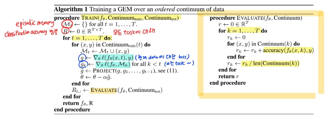
GEM의 핵심 특징 : “EPISODIC memory” ( \(\mathcal{M}_t\) )

• stores a “subset of observed examples” of task \(t\)

• 현실적으로 메모리 제약! total budget = \(M\)

  ( \(m=M/T\) memories for each task )

  ( 만약 task의 개수를 모를 경우, gradually reduce \(m\) )

• 목표 : minimize BACKWARD transfer ( catastrophic forgetting ), by using episodic memory

Loss at memories from the \(k\)-th task :

• \(\ell\left(f_{\theta}, \mathcal{M}_{k}\right)=\frac{1}{ \mid \mathcal{M}_{k} \mid } \sum_{\left(x_{i}, k, y_{i}\right) \in \mathcal{M}_{k}} \ell\left(f_{\theta}\left(x_{i}, k\right), y_{i}\right)\).

하지만, “현재 데이터의 loss”와 함께 “위의 memory의 loss function”을 둘 다 minimize하는 것은, \(\mathcal{M_k}\) 메모리에 저장된 데이터셋에 overfitting 위험!

따라서, 위의 loss (Loss at memories from the \(k\)-th task)는 inequality constraints로만 사용한다!

최종 목표 :

\(\begin{aligned} \operatorname{minimize}_{\theta} & \ell\left(f_{\theta}(x, t), y\right) \\ \text { subject to } & \ell\left(f_{\theta}, \mathcal{M}_{k}\right) \leq \ell\left(f_{\theta}^{t-1}, \mathcal{M}_{k}\right) \text { for all } k<t \end{aligned}\).

위 식을 효율적으로 풀고자 함.

• 1) old predictor \(f_{\theta}^{t-1}\) 를 저장할 필요가 없음

  ( 단지, 이전 task의 loss가 parameter update \(g\)이후 loss가 늘어나지 않음만 “확인”하면 되니까 )

• 2) 위의 “확인”은, loss gradient vector & proposed update 사이의 angle을 계산함으로써 가능

  • \(\left\langle g, g_{k}\right\rangle:=\left\langle\frac{\partial \ell\left(f_{\theta}(x, t), y\right)}{\partial \theta}, \frac{\partial \ell\left(f_{\theta}, \mathcal{M}_{k}\right)}{\partial \theta}\right\rangle \geq 0, \text { for all } k<t\).

위의 식을, Quadratic Program / dual problem / primal 등을 사용하여 정리하면, 최종적으로 아래와 같다.

\(\begin{aligned} \operatorname{minimize}_{z} & \frac{1}{2} z^{\top} z-g^{\top} z+\frac{1}{2} g^{\top} g \\ \text { subject to } & G z \geq 0, \end{aligned}\).

where \(G=-\left(g_{1}, \ldots, g_{t-1}\right)\)

\[\begin{aligned} \operatorname{minimize}_{v} & \frac{1}{2} v^{\top} G G^{\top} v+g^{\top} G^{\top} v \\ \text { subject to } & v \geq 0, \end{aligned}\]

4. Algorithm

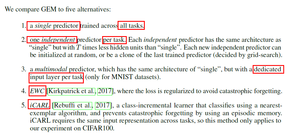
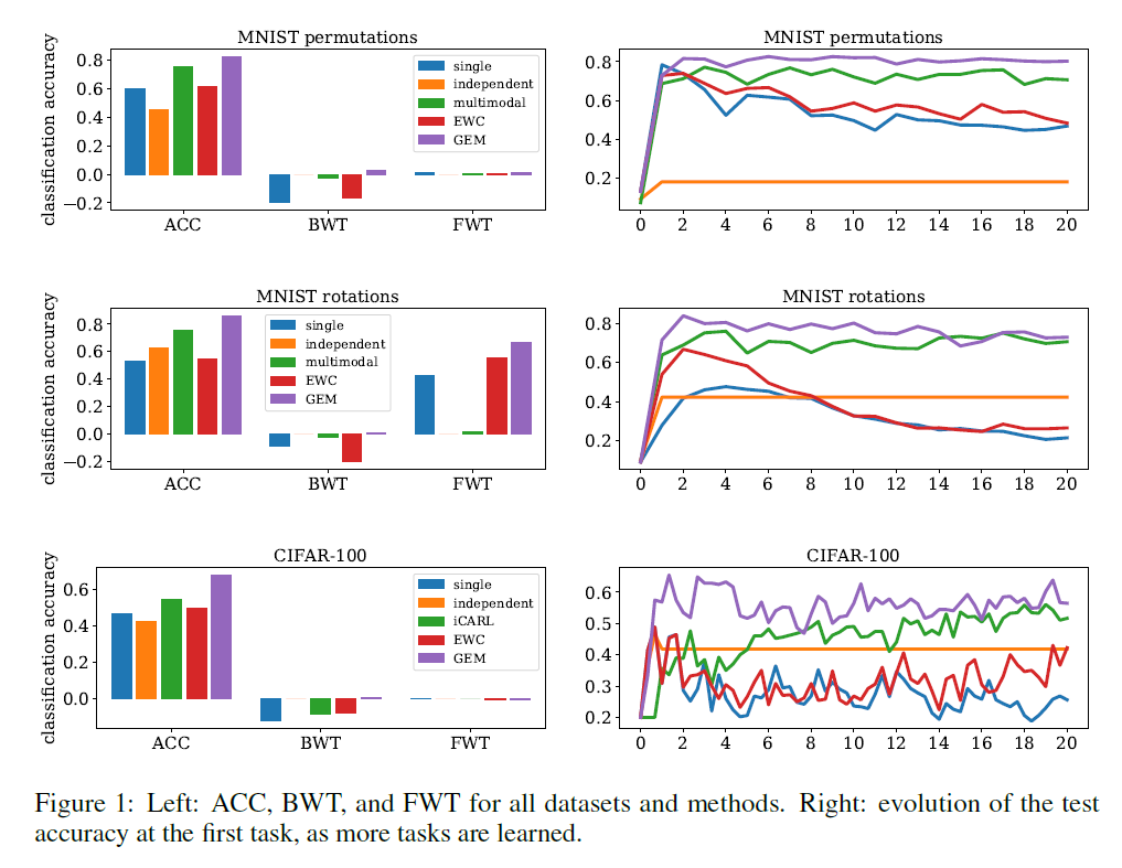
5. Experiments

사용한 데이터셋

( 모든 데이터셋에 대해 \(T = 20\) tasks )

• 1) MNIST Permutations
• 2) MNIST Rotations,
• 3) Incremental CIFAR100
  • each task introduces a new set of classes
  • For a total number of T tasks, each new task concerns examples from a disjoint subset of 100/T classes