[cs330] (2강) Multi-Task Learning, Transfer Learning Basics

Multi-Task Learning & Transfer Learning Basics

Standford CS330 수강 후 강의 내용 요약

1. Multi-Task Learning

(1) Notation

Single-task Learning (supervised)

• classification / regression 등의 단일 task

• dataset : \(\mathscr{D}=\left\{(\mathbf{x}, \mathbf{y})_{k}\right\}\)

• goal : minimize Loss function ( \(\min _{\theta} \mathscr{L}(\theta, \mathscr{D})\) )

  • ex) NLL (Negative Log Likelihood)

    \(\mathscr{L}(\theta, \mathscr{D})=-\mathbb{E}_{(x, y) \sim \mathscr{D}}\left[\log f_{\theta}(\mathbf{y} \mid \mathbf{x})\right]\).

Task에 대한 정의

• (\(i\)번째 Task)

  \(\quad \mathscr{T}_{i} \triangleq\left\{p_{i}(\mathbf{x}), p_{i}(\mathbf{y} \mid \mathbf{x}), \mathscr{L}_{i}\right\}\).

• 이 task를 풀기 위해 사용되는 dataset : \(\mathscr{D}_{i}^{t r}\) & \(\mathscr{D}_{i}^{\text {test }}\)

  ( 앞으로 \(\mathscr{D}_{i}^{t r}\)를 \(\mathscr{D}_{i}\) 로 표기할 것 )

(2) Examples of Tasks

하나의 단일 task (Single Task)를 푸는 것 외에, 여러 Task를 푸는 경우도 있다.

Multi-task Classification

• 사용하는 loss function ( ) 이 모든 task에 걸쳐서 동일하다

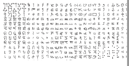
• ex) “언어 별” 글씨/단어 구분하기, “개인 별” 스팸문자 구분하기

  

Multi-label Learning

• 사용하는 loss function ( \(\mathscr{L}_{i}\) ) 과 데이터 분포 ( \(p_{i}(\mathbf{x})\) )이 모든 task에 걸쳐서 동일하다

• ex) 1000명의 사진에서, “안경”,”모자”,”쌍꺼풀” 여부 파악하기

  ex) scene understanding

  

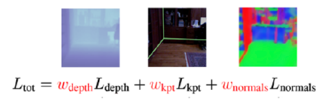
지금까지 살펴 본 위의 두 경우 모두, task가 다르다 하더라도 사용하는 loss function은 동일했다. 하지만, 아래와 같은 경우에에는, loss function 또한 task 별로 다를 수 있다.

• task의 Y label 들이 continuous, discrete로 혼재된 경우
• 여러 metric에 대해 신경쓰고 싶을 경우

(3) Conditioning on task label

우리는 결국 하나의 model로 여러 개의 task를 풀고 싶은 것이다. 직관적으로 생각했을때, 결국 task를 식별할 수 있는 task descriptor \(\mathbf{z}_{i}\)를 input으로 함께 넣어야 한다.

• (before) \(f_{\theta}(\mathbf{y} \mid \mathbf{x})\)
• (after) \(f_{\theta}\left(\mathbf{y} \mid \mathbf{x}, \mathbf{z}_{i}\right)\)

Task 별로 각자의 loss function이 있다고 할 경우, 가장 기본적인 형태의 objective (function)은 다음과 같이 나타낼 수 있다.

• \(\min _{\theta} \sum_{i=1}^{T} \mathscr{L}_{i}\left(\theta, \mathscr{D}_{i}\right)\).

결국, Multi-task learning의 핵심은 아래의 3가지 측면으로 요약할 수 있다.

• [model] 어떻게 \(\mathbf{z}_i\)에 대한 conditioning을 할 것인가?
• [objective] 어떠한 objective function을 사용할 것인가?
• [optimization] 어떻게 optimization을 할 것인가?

(4) Model

결국, 여러 task들을 수행하기 위해, “공통”으로 역할을 할 parameter와, “개별 task”의 역할을 할 parameter 2가지를 잘 구분하여 학습시키는 것이 핵심이다. 이 내용에서 풀고자하는 문제는 아래 2가지로 설명할 수 있을 것 같다.

Key Question

• Q1) How should the model be conditioned on \(\mathbf{z}_i\)?

• Q2 ) What parameters of the model should be shared ?

가장 극단적인 경우2가지 경우를 생각해보자.

(1) 단 하나의 parameter도 공유 하지 않는 경우

• 모든 task를 output나오기 직전까지 각자의 NN으로 학습한 뒤, 가장 마지막 단계에서 indicator function으로써 task에 대한 구분만 하는 모델이다

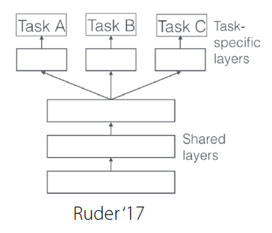
(2) (거의) 모든 parameter를 공유하는 경우

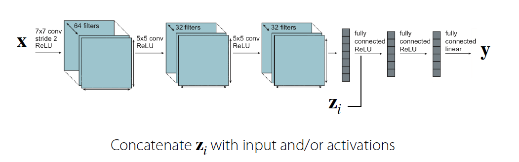
• 하나의 NN으로 계속 시작해서, 중간에 \(\mathbf{z}_i\)를 concatenate한다.

요약 : (1)와 (2) 사이 즈음에, “공통의 역할을 수행하는 부분에 대해서는 같은 parameter”를, “다른 부분을 수행하는 부분에는 다른 parameter”를 가지는 structure를 잘 만들어야한다!

Alternative View on the Multi-task architecture

위에서 다뤘던 내용은, 결국 “어떻게 parameter를 2개로 잘 나눌까?”이다.

“choosing how to condition on \(\mathbf{z}_i\) = choosing how & where to share parameters”

이러한 점에서, 우리의 objective를 다음과 같이 나타낼 수 있다.

\(\min _{\theta^{s h}, \theta^{1}, \ldots, \theta^{T}} \sum_{i=1}^{T} \mathscr{L}_{i}\left(\left\{\theta^{s h}, \theta^{i}\right\}, \mathscr{D}_{i}\right)\).

• \(\theta^{sh}\) : shared parameter
• \(\theta^{i}\) : 각 task의 parameter

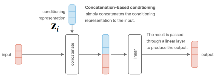
a) Concatenation-based conditioning

b) Additive conditioning

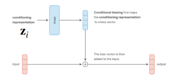
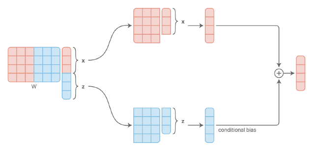
아래의 그림을 통해, a)와 b)는 사실상 동일한 방법임을 알 수 있다.

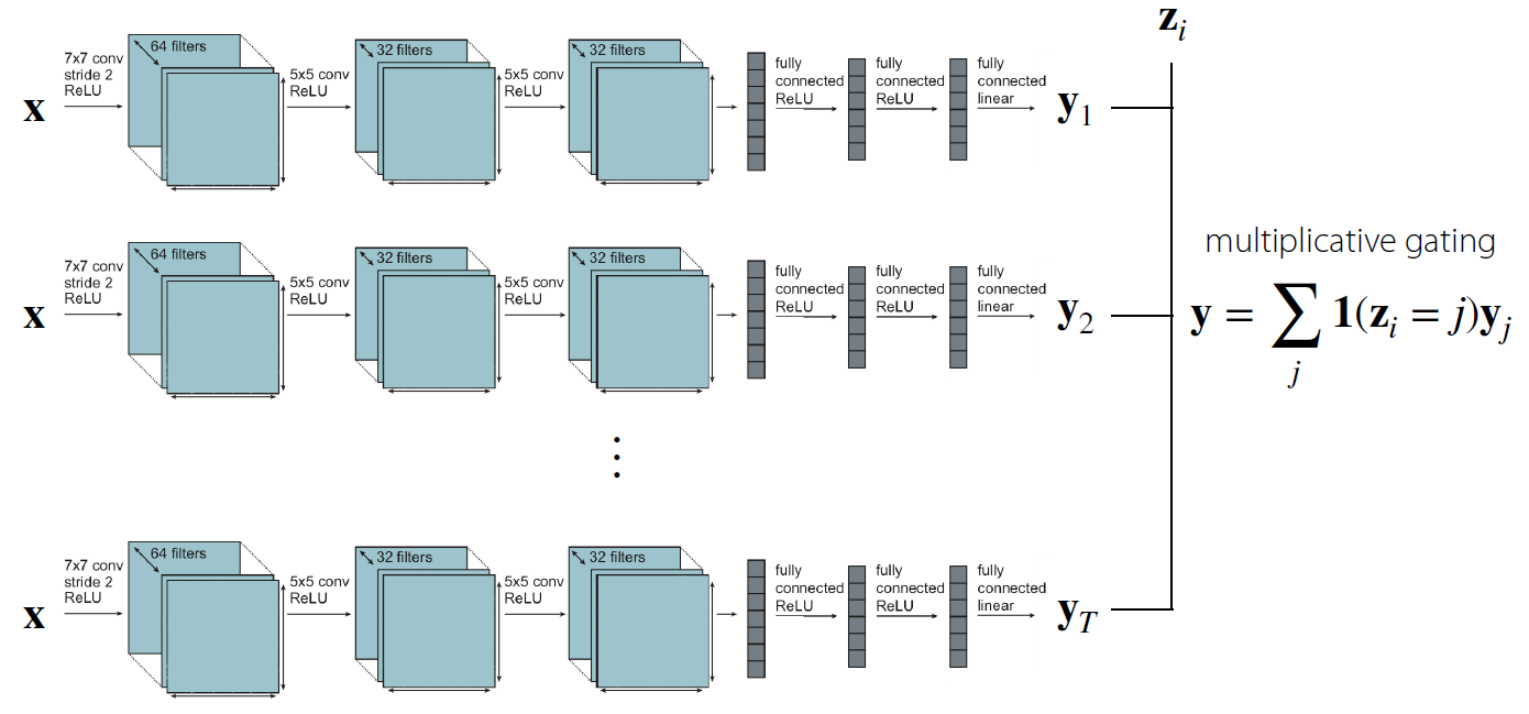
c) Multi-head architecture

d) Multiplicative conditioning

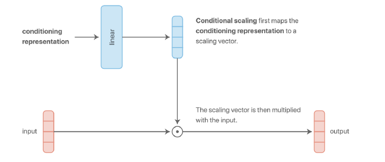
• 다른 conditioning 방법들 보다 더 expressive하다!

e) 그 외의 방법들…

그래서 결론은 무엇인가? 위의 architecture들 중 어느 것을 선택해야 하는가? 아쉽게도 정답은 없다. 어떠한 구조가 적절할지는 “문제에 따라 천차만별 (problem dependent)”하고, intuition이나 domain knowledge에 따라 다를 수 있기 때문이다.

(5) Optimization

가장 기본적인 형태의 objective ( Vanilla MTL Objective )는 아래와 같다.

• \(\min _{\theta} \sum_{i=1}^{T} \mathscr{L}_{i}\left(\theta, \mathscr{D}_{i}\right)\).

여기서 optimization을 수행하는 기본 frame은 아래와 같다.

1. Sample mini-batch of tasks \(\mathscr{B} \sim\left\{\mathscr{T}_{i}\right\}\)
2. Sample mini-batch datapoints for each task \(\mathscr{D}_{i}^{b} \sim \mathscr{D}_{i}\)
3. Compute loss on the mini-batch: \(\hat{\mathscr{L}}(\theta, \mathscr{B})=\sum_{\mathscr{T}_{k} \in \mathscr{B}} \mathscr{L}_{k}\left(\theta, \mathscr{D}_{k}^{b}\right)\)
4. Backpropagate loss to compute gradient \(\nabla_{\theta} \hat{\mathscr{L}}\)
5. Apply gradient with your favorite neural net optimizer (e.g. Adam)

주의할 점!

• 1단계에서 task를 샘플링할 때 “데이터 크기와 무관하게 Uniform하게” 해야한다!
• regression task를 푸는 경우, task label들의 scale을 서로 맞춰준다.

(6) Challenges

아래와 같은 2가지 어려움이 있을 수 있다.

• 1) Negative Transfer
• 2) Overfitting

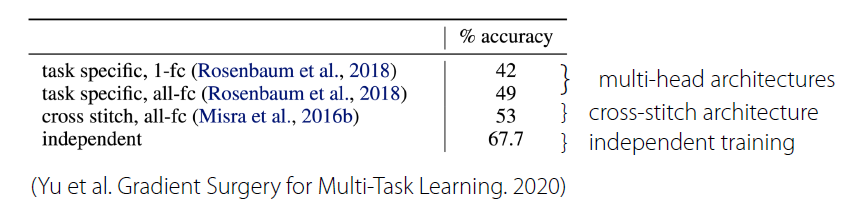
Negative Transfer

여러 task를 하나의 모델보다, 각 task에 각각의 independent한 모델로 문제를 푸는것이 더 나을 수 있다

즉, parameter를 서로 공유하지 않는 것이 더 낫다는 것이다 ( task들 간의 공통의 structure가 없는 경우를 의미할 것이다 )

• ex) Multi-Task CIFAR-100

  

Negative Transfer가 발생하는 이유?

• 1) Optimization challenges
  • task간에 서로 간섭(방해)가 이루어짐 ( cross-task interference )
  • task별로 다른 적절한 learning rate
• 2) Limited Representation
  • multi-task NN의 경우, single-task의 경우보다 더 large capacity 필요

해결하기 위해서?

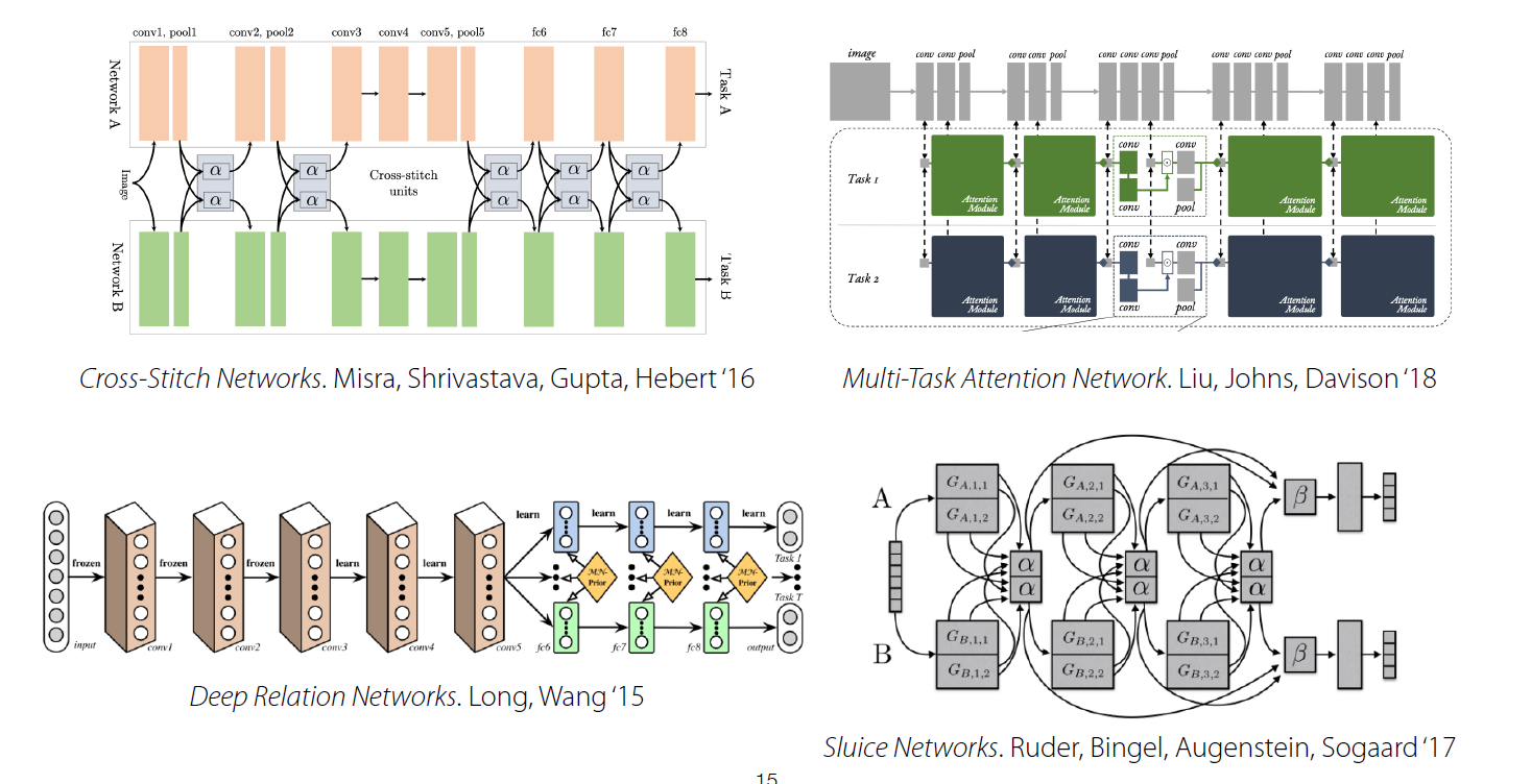
• “더 적은” parameter를 share해야 한다.

  ( share를 할지/안할지의 binary한 문제가 아니다! )

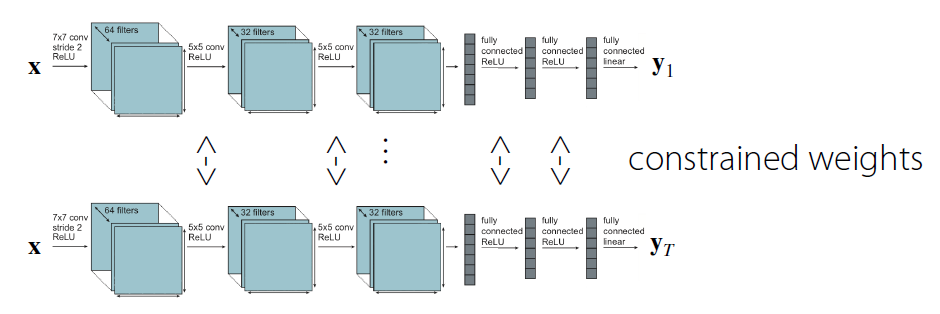
• ex) Soft parameter sharing

  • weight들이 서로 유사하도록 constraint를 부여한다.
  • \(\min _{\theta^{\text {sh }}, \theta^{1}, \ldots, \theta^{T}} \sum_{i=1}^{T} \mathscr{L}_{i}\left(\left\{\theta^{s h}, \theta^{i}\right\}, \mathscr{D}_{i}\right)+\underbrace{\sum_{t^{\prime}=1}^{T}\left\|\theta^{t}-\theta^{\prime}\right\|}_{\text {"Soft parameter sharing' }}\).

  

Overfitting

parameter를 충분히 share하지 않았기 때문에, 특정 task에 대해 overfitting이 발생할 수 있다. 따라서 해결방법은 Negative Transfer와 정반대이다. 더 많은 parameter를 share하도록 architecture를 짜면 된다.

2. Case Study

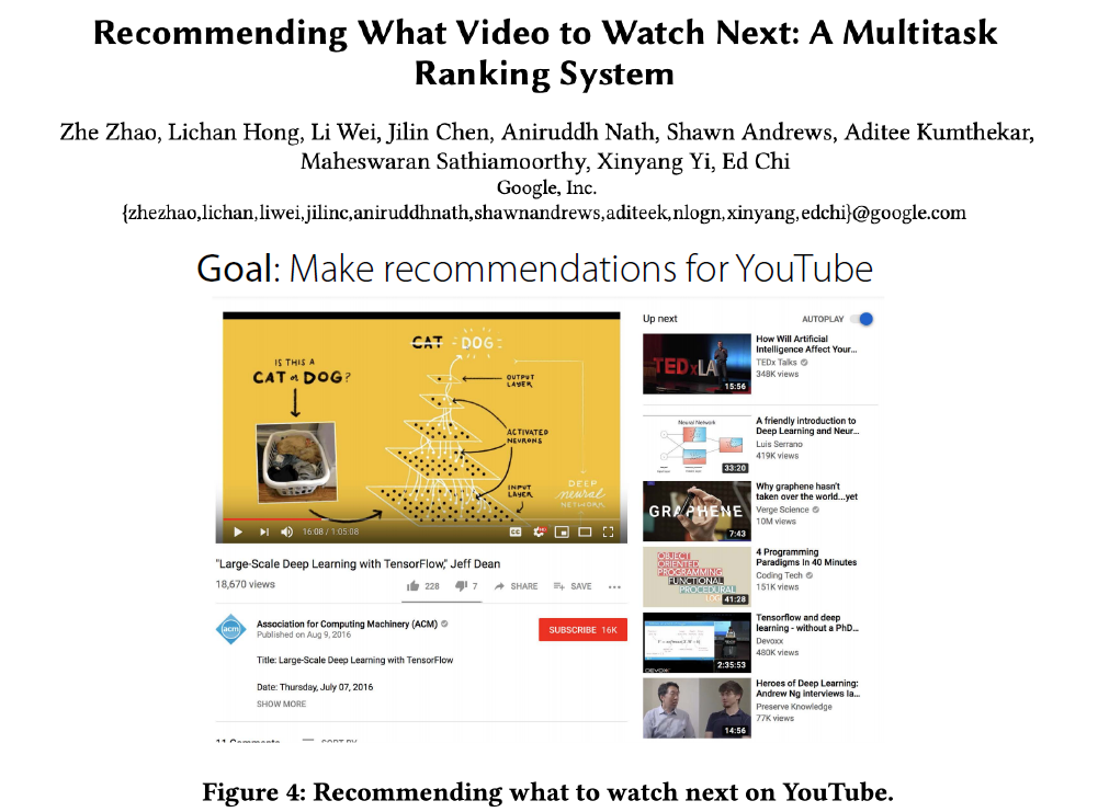
(1) Goal

목표는 유저에게 Youtube 영상 추천을 해주는 것이다.

하지만, 영상 추천에 있어서 아래와 같은 여러가지의 상충되는 objective가 존재한다.

• 1) “가장 평점을 높게 줄” 영상 추천하기
• 2) “가장 share(공유)를 많이 할 법한” 영상 추천하기
• 3) “가장 시청할 법한” 영상 추천하기

위 세가지 objective는 서로 다르나, 공통으로 “좋아할 만한/관심 가질만한 영상”이라는 공통의 structure를 가진다고 볼 수 있다.

( 다만, 위 목표에는 어쩔 수 없는 implicit bias가 존재한다. “좋아해서” 본 영상일 수도 있지만, “추천 받아서 본 영상”일 수도 있기 때문이다! )

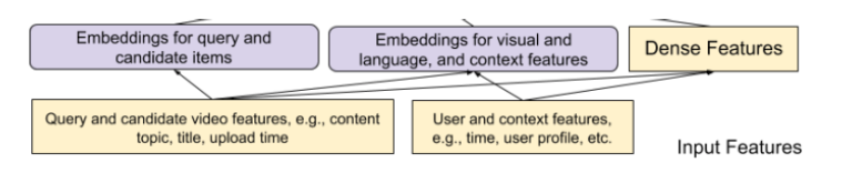
(2) Framework

위 recommendation model을 위한 input으로는,

• (1) 현재 시청하고 있는 동영상 ( current watching video (query video) )
• (2) 유저의 정보/특징 ( user feature )

이 들어간다.

그런 뒤, 아래와 같은 step으로 추천이 진행된다.

• step 1) Generate a few hundred of candidate videos

  ( Candidate video : 여러 candidate generation algorithm에서 video들을 뽑아낸다 )

• step 2) Rank candidate

• step 3) Serve top ranking video to user

(3) Ranking Problem

Input :

Output :

• 1) engagement and 2) satisfaction with candidate video

1) Engagment

• (binary classification task의 경우) click 수
• (regression task의 경우) 영상 시청 시간

2) Satisfaction

• (binary classification task의 경우) like수
• (regression task의 경우) 평점 (rating)

Ranking Score는 위 1) Engagement와 2) Satisfaction의 weighted sum으로 manual하게 정할 수 있다.

(4) Architecture

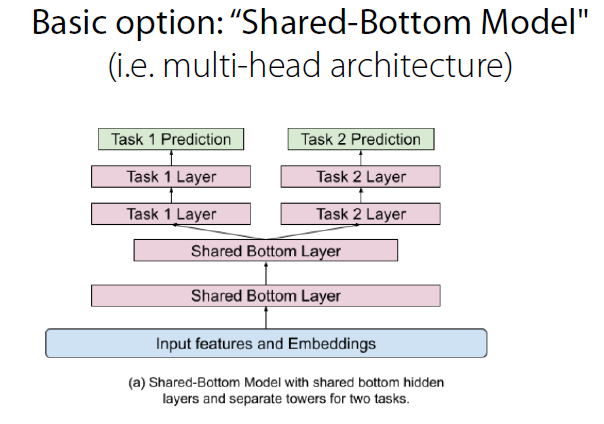
• 만약 task들 사이의 correlation이 낮으면 좋지 않은 구조일 수 있다.

Multi-gate Mixture of Experts (MMoE)

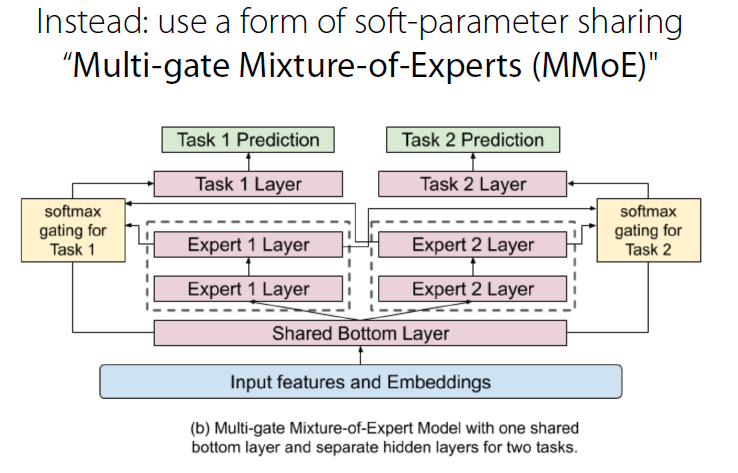
• 다른 부분의 NN가 자기 역할 잘 하도록 (specialize)!

  \(\rightarrow\) called “expert NN”, \(f_i(x)\)

• input \(x\)와 task \(k\)에 대해, 어떠한 expert NN를 사용할지 결정

  \(\rightarrow\) \(g^{k}(x)=\operatorname{softmax}\left(W_{g^{k}} x\right)\).

• 선택된 expert로부터 feature 계산

  \(\rightarrow\) \(f^{k}(x)=\sum_{i=1}^{n} g_{(i)}^{k}(x) f_{i}(x)\).

• output 계산

  \(\rightarrow\) \(y_{k}=h^{k}\left(f^{k}(x)\right)\).

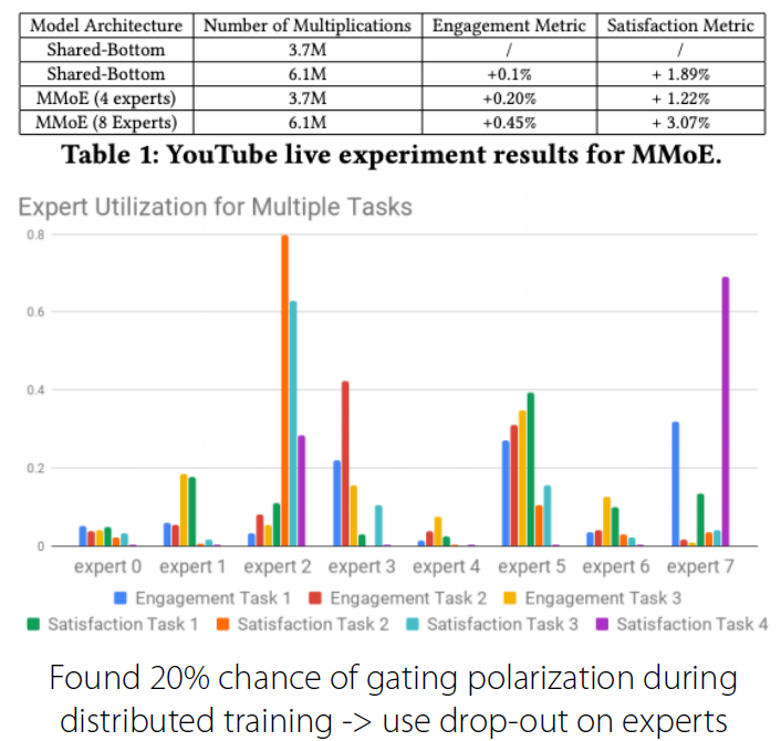
(5) Experiments

3. Multi-task Learning vs Transfer Learning

Multi Task learning

• 여러 task ( \(\mathscr{T}_{1}, \cdots, \mathscr{T}_{T}\) ) 를 “한번에” 해결
• goal :

Transfer Learning

• (선) source task \(\mathscr{T}_{a}\) 풀기

  (후) target task \(\mathscr{T}_{b}\) 풀기

  ( with knowledge learned from \(\mathscr{T}_{a}\) )

• 가정 ) transfer 중 \(\mathscr{D}_{a}\) 사용 불가

4. Meta Learning

(1) Two ways to view meta learning

a) Mechanistic view

• 전체 데이터를 input으로 받아 output을 내는 DNN
• 모든 task의 dataset들을 포함하는 meta-dataset을 사용하여 이 DNN을 학습시킴

b) Probabilistic View

• 여러 task들로 부터 prior knowledge를 뽑아냄
• 해당 prior knowledge를 사용하여 posterior 추정

우리는 a) Mechanistic View의 관점에서 문제를 바라볼 것이다.

(2) Problem Definitions

Supervised Learning

\(\begin{array}{l} \underset{\phi}{\arg \max } \log p(\phi \mid \mathcal{D}) \\ =\arg \max _{\phi} \log p(\mathcal{D} \mid \phi)+\log p(\phi)\\ =\arg \max _{\phi} \sum_{i} \log p\left(y_{i} \mid x_{i}, \phi\right)+\log p(\phi) \end{array}\).

• 위 모델의 문제점은? data가 충분하지 않은 경우 BAD

Additional data를 추가할 수 없을까?

\(\arg \max _{\phi} \log p\left(\phi \mid \mathcal{D}, \mathcal{D}_{\text {meta-train }}\right)\).

• \(\mathcal{D}=\left\{\left(x_{1}, y_{1}\right), \ldots,\left(x_{k}, y_{k}\right)\right\}\) : 지금 풀고자하는 task의 dataset
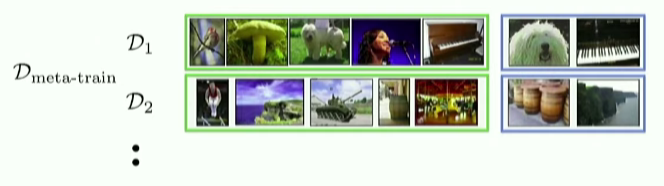
• \(\mathcal{D}_{\text {meta-train }}=\left\{\mathcal{D}_{1}, \ldots, \mathcal{D}_{n}\right\}\) : 이용하고자 하는 기존 task들의 dataset들
• \(\mathcal{D}_{i}=\left\{\left(x_{1}^{i}, y_{1}^{i}\right), \ldots,\left(x_{k}^{i}, y_{k}^{i}\right)\right\}\).

위 식에서, \(\mathcal{D}_{\text {meta-train }}\)를 데이터 그대로 계속 들고다니며 사용하지 않을 수 없을까?

\(\rightarrow\) meta parameter ( \(\theta\) )를 학습한 뒤 그것을 사용하자!

\(\theta: p\left(\theta \mid \mathcal{D}_{\text {meta-train }}\right)\).

\(\begin{aligned} \log p\left(\phi \mid \mathcal{D}, \mathcal{D}_{\text {meta-train }}\right) &=\log \int_{\Theta} p(\phi \mid \mathcal{D}, \theta) p\left(\theta \mid \mathcal{D}_{\text {meta-train }}\right) d \theta \\ & \approx \log p\left(\phi \mid \mathcal{D}, \theta^{\star}\right)+\log p\left(\theta^{\star} \mid \mathcal{D}_{\text {meta-train }}\right) \end{aligned}\).

여기서 \(\theta^{\star}=\arg \max _{\theta} \log p\left(\theta \mid \mathcal{D}_{\text {meta-train }}\right)\)를 meta-learning이라고 한다.

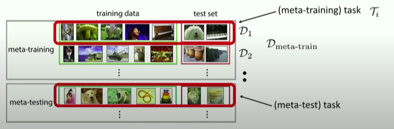
(3) Example

전체 학습 알고리즘은 아래의 2가지로 이루어진다고 볼 수 있다.

• 1) meta-learning : \(\theta^{\star}=\arg \max _{\theta} \log p\left(\theta \mid \mathcal{D}_{\text {meta-train }}\right)\).
• 2) adaptation : \(\phi^{\star}=\arg \max _{\phi} \log p\left(\phi \mid \mathcal{D}, \theta^{\star}\right)\).

전체 Structure

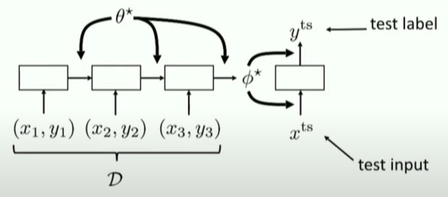
Meta-tranining time

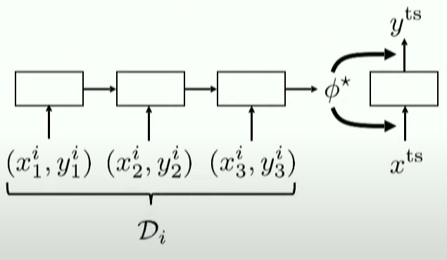
따라서, 우리는 task별로 test set을 남겨놔야한다!

\(\begin{array}{l} \mathcal{D}_{\text {meta-train }}=\left\{\left(\mathcal{D}_{1}^{\mathrm{tr}}, \mathcal{D}_{1}^{\mathrm{ts}}\right), \ldots,\left(\mathcal{D}_{n}^{\mathrm{tr}}, \mathcal{D}_{n}^{\mathrm{ts}}\right)\right\} \\ \mathcal{D}_{i}^{\operatorname{tr}}=\left\{\left(x_{1}^{i}, y_{1}^{i}\right), \ldots,\left(x_{k}^{i}, y_{k}^{i}\right)\right\} \\ \mathcal{D}_{i}^{\mathrm{ts}}=\left\{\left(x_{1}^{i}, y_{1}^{i}\right), \ldots,\left(x_{l}^{i}, y_{l}^{i}\right)\right\} \end{array}\).

Summary

위의 meta-learning & adaptation 단계는 아래와 표현할 수도 나타낼 수 있다.

\(\phi^{\star}=f_{\theta^{\star}}\left(\mathcal{D}^{\mathrm{tr}}\right)\).

learn \(\theta\) such that \(\phi=f_{\theta}\left(\mathcal{D}_{i}^{\mathrm{tr}}\right)\) is good for \(\mathcal{D}_{i}^{\mathrm{ts}}\)

\(\theta^{\star}=\max _{\theta} \sum_{i=1}^{n} \log p\left(\phi_{i} \mid \mathcal{D}_{i}^{\mathrm{ts}}\right)\).