( 참고 : 패스트 캠퍼스 , 한번에 끝내는 컴퓨터비전 초격차 패키지 )
Representation Learning (3)
3. Unsupervised Representation Learning
(4) Place Recognition
1. NetVLAD (2016)
( NetvLAD : CNN architecture for weakly supervised place recognition, Arandjelovic et al., CVPR 2015 )
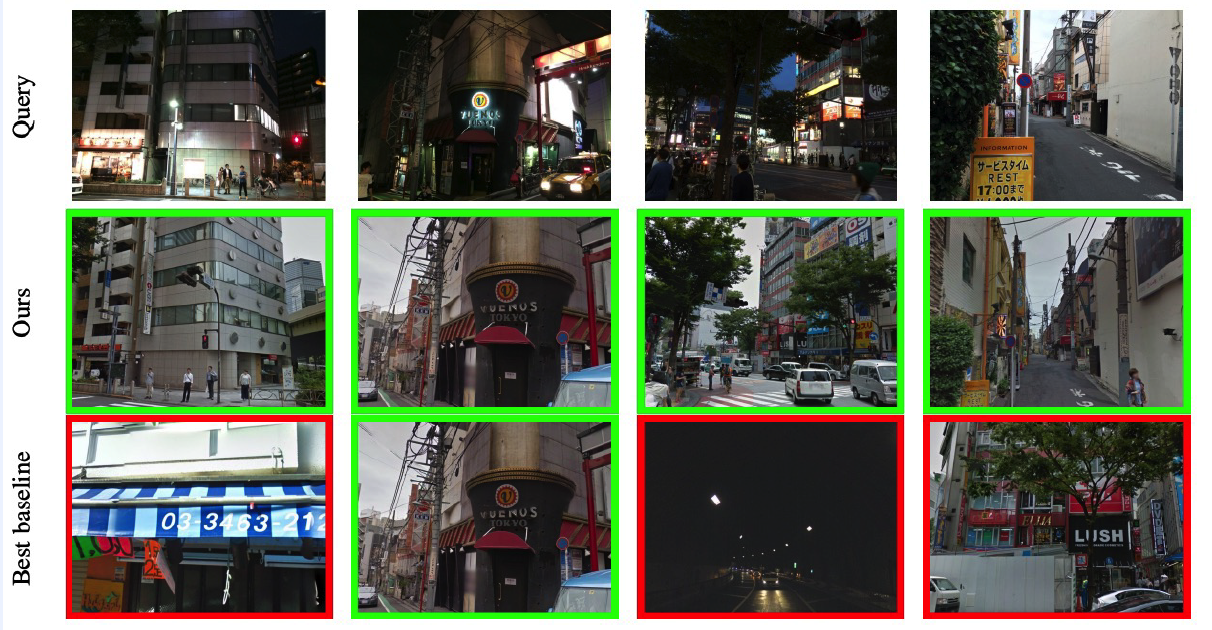
(1) Visual Place Recognition
- finding place image, given query image
- challenges
- same place, but different camera pose/illumination, occlusion, truncation….
(2) Solution
- solve by instance-level image retrieval
- Find image descriptor
(3) Contributions
- Hand-engineering \(\rightarrow\) CNN features
- large dataset from Google street view
- End-to-end training, using time machine images
(4) NetVLAD : A generalized VLAD layer
- VLAD = Vector of Locally Aggregated Descriptors
- widely used in instance-level retrieval / classificaiton
- NetVLAD = (cnn)Network + VLAD

(5) Weakly-supervised Ranking Loss
- Triplet-set
- \(\left(q,\left\{p_{i}^{q}\right\},\left\{n_{j}^{q}\right\}\right)\).
- positive = closest from query ( based on GPS (lat,long) )
- \(p_{i *}^{q}=\underset{p_{i}^{q}}{\operatorname{argmin}} d_{\theta}\left(q, p_{i}^{q}\right)\).
- Triplet-loss : \(d_{\theta}\left(q, p_{i *}^{q}\right)\).
- Loss function : \(L_{\theta}=\sum_{j} l\left(\min _{i} d_{\theta}^{2}\left(q, p_{i}^{q}\right)+m-d_{\theta}^{2}\left(q, n_{j}^{q}\right)\right)\)
Why “weakly” supervised?
- Do not have “real positive”…just treat “closests image based on GPS” as positive!
Code
- https://github.com/Nanne/pytorch-NetVlad/blob/master/netvlad.py
class NetVLAD(nn.Module):

    def __init__(self, num_clusters=64, dim=128,
                 normalize_input=True, vladv2=False):

        super(NetVLAD, self).__init__()
        self.num_clusters = num_clusters # K
        self.dim = dim # N ( = H x W )
        self.alpha = 0
        self.vladv2 = vladv2 $$ vladv1 or vladv2
        self.normalize_input = normalize_input
        self.conv = nn.Conv2d(dim, num_clusters, kernel_size=(1, 1), bias=vladv2) #1d-conv
        self.centroids = nn.Parameter(torch.rand(num_clusters, dim))

    def init_params(self, clsts, traindescs):

        if self.vladv2 == False:
            clstsAssign = clsts / np.linalg.norm(clsts, axis=1, keepdims=True)
            dots = np.dot(clstsAssign, traindescs.T)
            dots.sort(0)
            dots = dots[::-1, :] # sort, descending
            self.alpha = (-np.log(0.01) / np.mean(dots[0,:] - dots[1,:])).item()
            self.centroids = nn.Parameter(torch.from_numpy(clsts))
            self.conv.weight = nn.Parameter(torch.from_numpy(self.alpha*clstsAssign).unsqueeze(2).unsqueeze(3))
            self.conv.bias = None
        else:
            knn = NearestNeighbors(n_jobs=-1)
            knn.fit(traindescs)
            del traindescs
            dsSq = np.square(knn.kneighbors(clsts, 2)[1])
            del knn
            self.alpha = (-np.log(0.01) / np.mean(dsSq[:,1] - dsSq[:,0])).item()
            self.centroids = nn.Parameter(torch.from_numpy(clsts))
            del clsts, dsSq

            self.conv.weight = nn.Parameter(
                (2.0 * self.alpha * self.centroids).unsqueeze(-1).unsqueeze(-1)
            )
            self.conv.bias = nn.Parameter(
                - self.alpha * self.centroids.norm(dim=1)
            )

    def forward(self, x):
        N, C = x.shape[:2] # WxH = N
				K = self.num_clusters # K

        if self.normalize_input:
            x = F.normalize(x, p=2, dim=1)

        # (1) soft-assignment
        soft_assign = self.conv(x).view(N, K, -1) # reshape with 1d-conv
        soft_assign = F.softmax(soft_assign, dim=1)

        x_flatten = x.view(N, C, -1)

        # (2) calculate residuals to each clusters (K)
        vlad = torch.zeros([N, K, C], dtype=x.dtype, layout=x.layout, device=x.device)
        for C in range(K): # slower than non-looped, but lower memory usage
            residual = x_flatten.unsqueeze(0).permute(1, 0, 2, 3) - \
                    self.centroids[C:C+1, :].expand(x_flatten.size(-1), -1, -1).permute(1, 2, 0).unsqueeze(0)
            residual *= soft_assign[:,C:C+1,:].unsqueeze(2)
            vlad[:,C:C+1,:] = residual.sum(dim=-1)

        vlad = F.normalize(vlad, p=2, dim=2)  # intra-normalization
        vlad = vlad.view(x.size(0), -1)  # flatten
        vlad = F.normalize(vlad, p=2, dim=1)  # L2 normalize (dim=0 : Batch)

        return vlad
2. DELF (Deep Local Features) (2017)
(1) Landmark Recognition
- same setting as visual place recognition*
- but more place! ( = large scale image retrieval )
(2) Algorithm
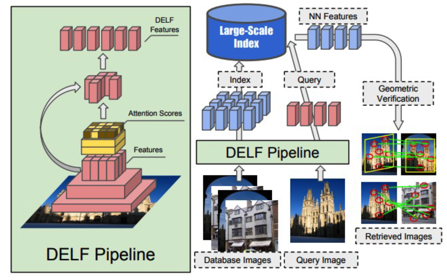
- embed both (1) index & (2) query image
- find nearest samples from large-scale index
(3) Image retrieval with DELF
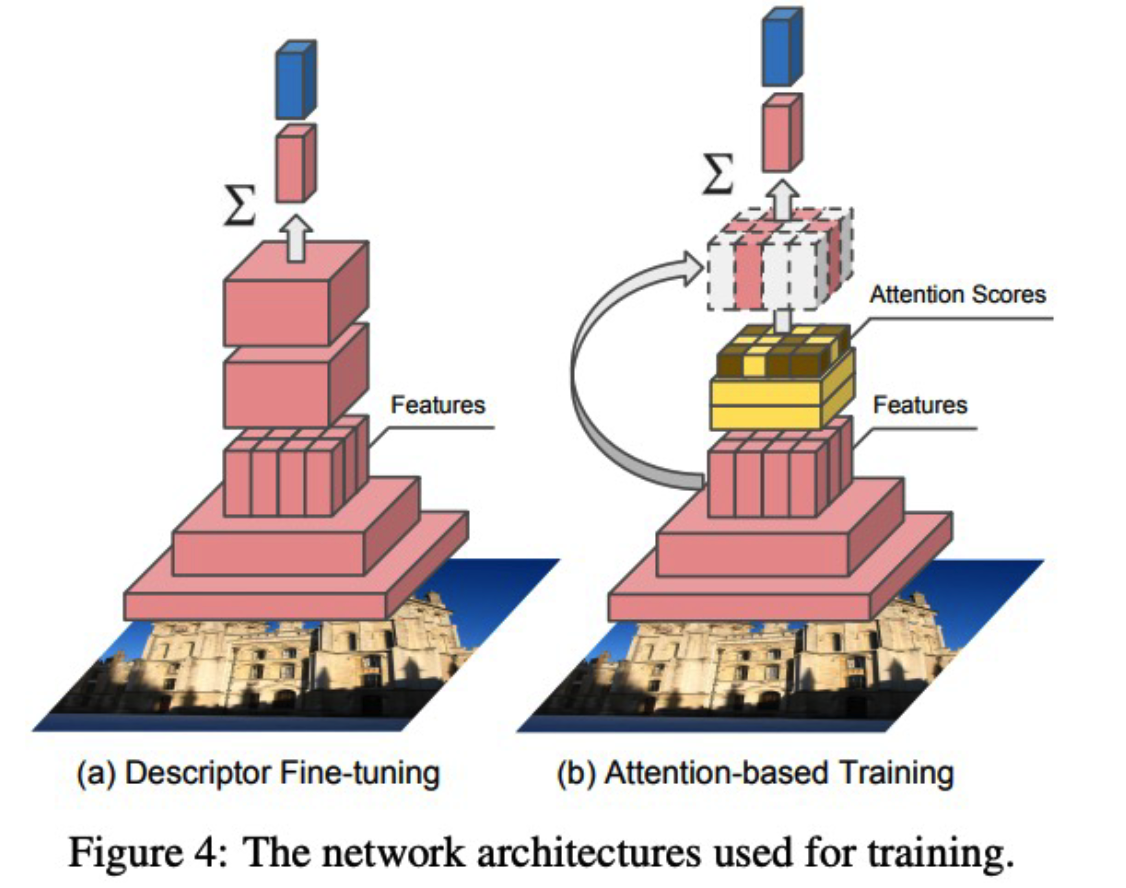
- step 1) Dense Localized Feature Extraction
- with clean images
- step 2) Attention-based Keypoint Selection
- with dirty images
- Loss ) CE loss
(3) Google Landmark Dataset
- 1,060,709 images from 12,894 landmarks
- 111,036 additional query
(4) Result
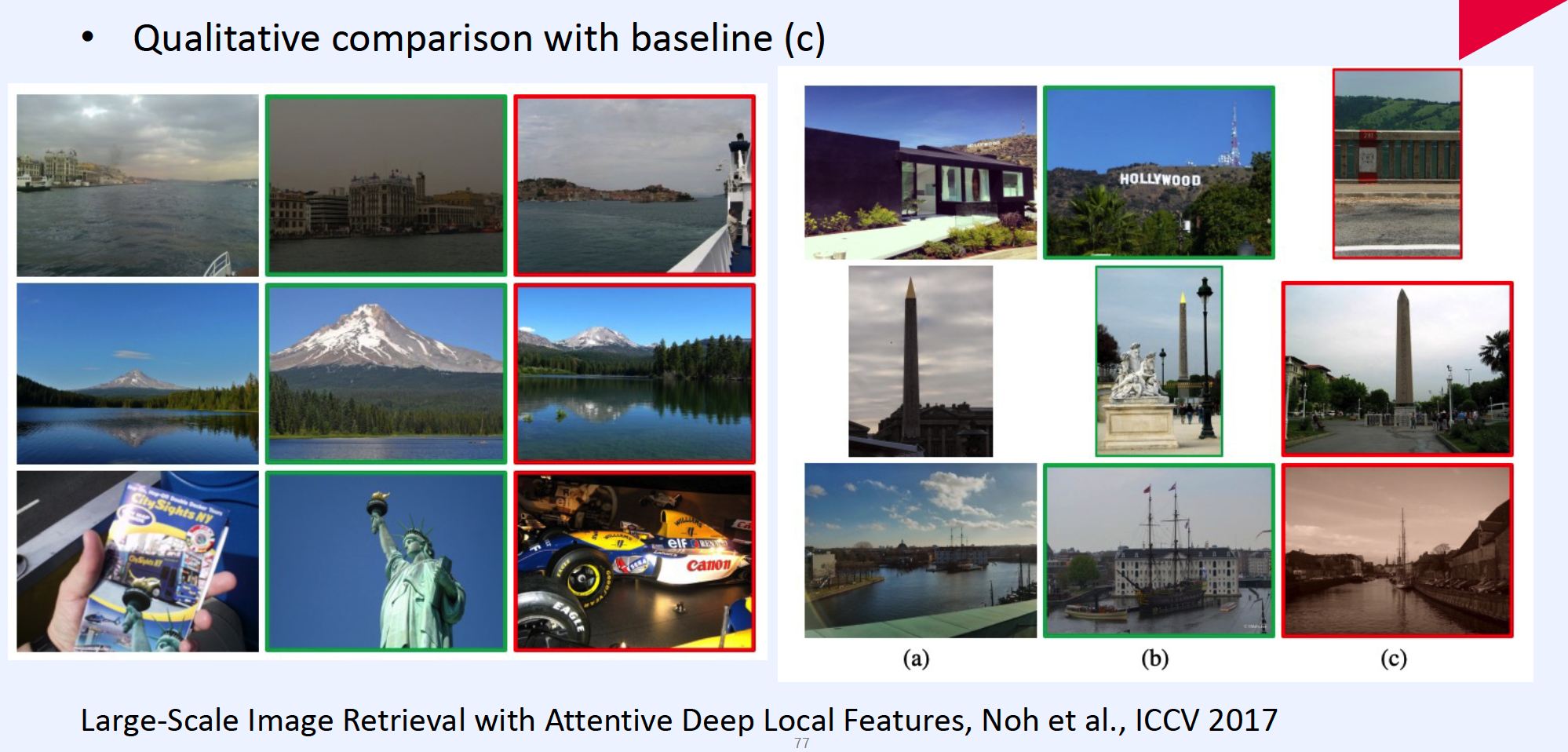
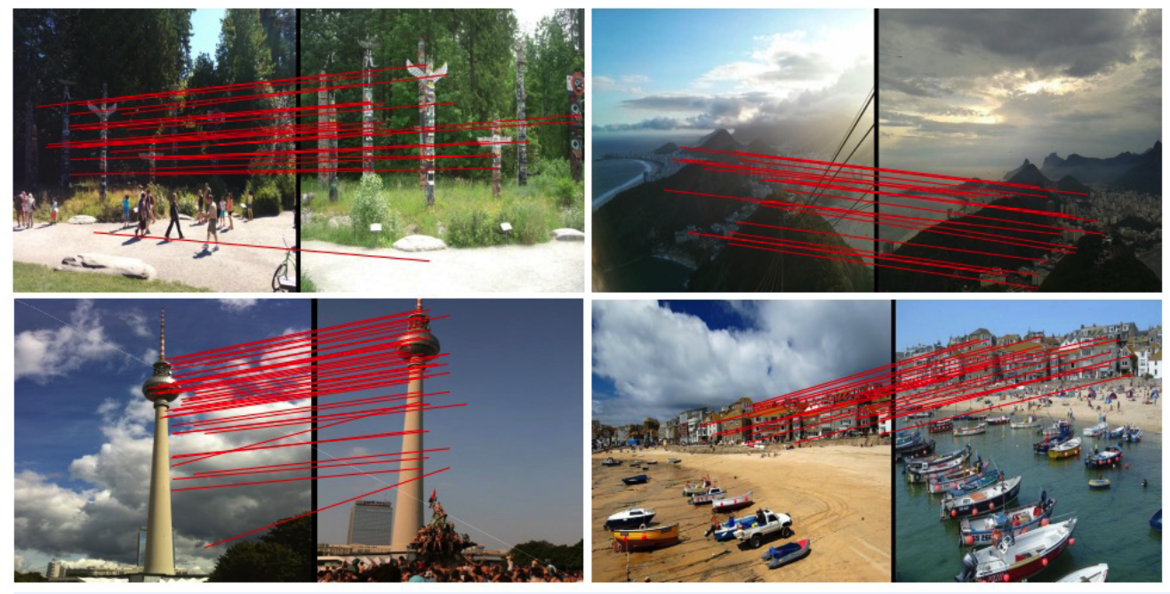
Visualization of feature correspondence & keypoint selection
