Time-Series Representation Learning via Temporal and Contextual Contrasting

Abstract
Introduction
Methods
1. TS Data Augmentation
2. Temporal Contrasting
3. Contextual Contrasting
Experiments
1. Experiment Setups
2. Results

0. Abstract

propose an unsupervised TS-TCC

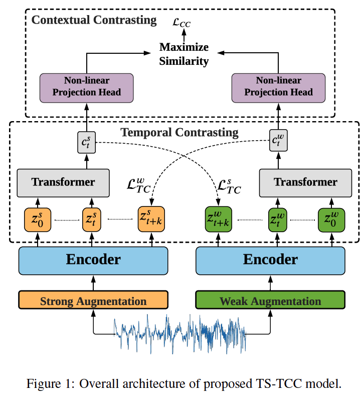
Time-Series representation learning framework via Temporal and Contextual Contrasting
(1) raw TS are transformed with 2 data augmentations
- weak augmentation
- strong augmentation
(2) novel temporal contrasting module
- to learn robust temporal representation
- by designing cross-view prediction
(3) propose contextual contrasting module
- to learn discriminative respresentations

1. Introduction

Contrastive Learning

mostly done in CV
but not in TS

Why not in TS?

(1) may not be able to address the temporal dependencies of data
(2) some augmentation techniques generally cannot fit well with TS

propose TS-TCC

employs simple & effective data augmentations
propose novel temporal contrastive module
propose contextual contrasting module

2. Methods

(1) TS Data Augmentation

Using different augmentations can improve robustness of learned representations

Augmentation

weak : jitter-and-scale
- jitter = add random variations to the signal
- scale = scale up its magnitude
strong : permutation-and-jitter
- permutation : split the signal into random # of segments ( max # = M ) & random shuffle
- jitter = random jittering

Notation

input sample : \(x\)
- strongly augmented view : \(x^s \sim \mathcal{T}_s\)
- weakly augmented view : \(x^w \sim \mathcal{T}_w\)
encoder : \(\mathbf{z}=f_{\text {enc }}(\mathbf{x})\)
- where \(\mathbf{z}=\left[z_1, z_2, \ldots z_T\right]\)
  - strongly augmented view : \(\mathbf{z}^s\)
  - weakly augmented view : \(\mathbf{z}^w\)

(2) Temporal Contrasting

given latent variable \(\mathbf{z}\),

use autoregressive model \(f_{a r}\) to summarize all \(\mathbf{z}_{\leq t}\) into a context vector \(c_t=f_{a r}(\mathbf{z} \leq t), c_t \in \mathbb{R}^h\)

\(c_t\) is used to predict the timesteps from \(z_{t+1}\) until \(z_{t+k}(1<k \leq K)\)
use log-bilinear model
- \(f_k\left(x_{t+k}, c_t\right)=\exp \left(\left(\mathcal{W}_k\left(c_t\right)\right)^T z_{t+k}\right)\).

Cross-view prediction task

use \(c_t^s\) to predict future timesteps of weak augmentation \(z_{t+k}^w\)
use \(c_t^w\) to predict future timesteps of strong augmentation \(z_{t+k}^s\)

Contrastive Loss

minimize dot product between the predicted representation & true one of same sample
maximize dot product with other samples \(\mathcal{N}_{t,k}\)

\(\begin{aligned} &\mathcal{L}_{T C}^s=-\frac{1}{K} \sum_{k=1}^K \log \frac{\exp \left(\left(\mathcal{W}_k\left(c_t^s\right)\right)^T z_{t+k}^w\right)}{\sum_{n \in \mathcal{N}_{t, k}} \exp \left(\left(\mathcal{W}_k\left(c_t^s\right)\right)^T z_n^w\right)} \\ &\mathcal{L}_{T C}^w=-\frac{1}{K} \sum_{k=1}^K \log \frac{\exp \left(\left(\mathcal{W}_k\left(c_t^w\right)\right)^T z_{t+k}^s\right)}{\sum_{n \in \mathcal{N}_{t, k}} \exp \left(\left(\mathcal{W}_k\left(c_t^w\right)\right)^T z_n^s\right)} \end{aligned}\).

Use transformer as the AR model

(3) Contextual Contrasting

to learn more discriminative representations
\(2N\) contexts
- positive pair : \(\left(c_t^i, c_t^{i^{+}}\right)\)
- negative pair : remaining \((2 N-2)\) pairs
loss function :
- \(\mathcal{L}_{C C}=-\sum_{i=1}^N \log \frac{\exp \left(\operatorname{sim}\left(c_t^i, c_t^{i^{+}}\right) / \tau\right)}{\sum_{m=1}^{2 N} \mathbb{1}_{[m \neq i]} \exp \left(\operatorname{sim}\left(c_t^i, c_t^m\right) / \tau\right)}\),
  - where \(\operatorname{sim}(\boldsymbol{u}, \boldsymbol{v})=\boldsymbol{u}^T \boldsymbol{v} / \mid \mid \boldsymbol{u} \mid \mid \mid \mid \boldsymbol{v} \mid \mid\)
Overall self-supervised loss :
- \(\mathcal{L}=\lambda_1 \cdot\left(\mathcal{L}_{T C}^s+\mathcal{L}_{T C}^w\right)+\lambda_2 \cdot \mathcal{L}_{C C}\).

3. Experiments

Experiment Setups
1. Datasets
2. Implementation Details
Results
1. Comparison with Baselines
2. Semi-supervised Training
3. Transfer Learning
4. Ablation Study

(1) Experiment Setups

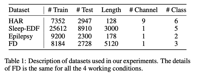
a) Datasets

3 public datasets + 1 additional dataset ( for transfer learning )

HAR (Human Activity Recognition)
- 30 subjects
- num classes = 6 activities
Sleep-EDF (Sleep Stage Classification)
- num classes = 5 EEG signals ( W, N1, N2, N3, REM )
Epilepsy (Epilepsy Seizure Prediction)
- 500 subjects
- num classes = 5 \(\rightarrow\) 2
  
  ( 4 of them do not include epileptic seizure \(\rightarrow\) group them into 1 class )
FD (Fault Diagnosis)
- for transferability experiment
- num domains = 4 different working conditions ( A, B, C, D )
- num classes = 3 class ( per each domain )
  - inner fault / outer fault / healthy

b) Implementation Details

train/val/tes : 60/20/20
etc) SleepEDF : subject-wise split
repeat experiment for 5 times ( 5 different seed )
- report mean & std
epochs : 40

( both for pretraining & downstream tasks )
batch size : 128 ( 32 for few-labeled data experiments )
Adam optimizer

(2) Results

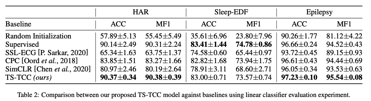
a) Comparison with Baselines

Baselines

(1) Random Initialization:
- training a linear classifier on top of frozen and randomly initialized encoder
(2) Supervised:
- supervised training of both encoder and classifier
(3) SSL-ECG
(4) CPC
(5) SimCLR
- use our timeseries specific augmentations to pretrain SimCLR

[ standard linear benchmarking evaluation scheme ]

To evaluate the performance of SSL-ECG, CPC, SimCLR and TS-TCC ….

step 1) pretrain ( w.o labeled data )
step 2) evaluation ( with a portion of the labeled data )
- standard linear evaluation scheme
- train a linear classifier on top of a frozen SSL pretrained encoder model

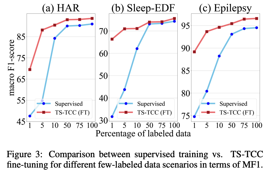
b) Semi-supervised Training

semi-supervised settings

by training ( = fine-tuning ) the model with 1%, 5%, 10%, 50%, and 75%

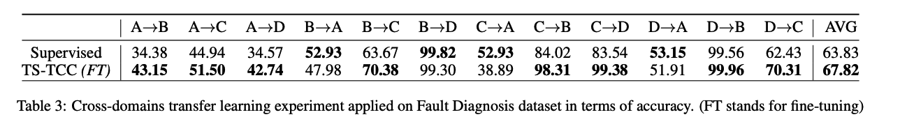
c) Transfer Learning

use Fault Diagnosis (FD) dataset
adopt 2 training schemes on the source domain
- (1) supervised training
- (2) TS-TCC fine-tuning
  - fine tune the pre-trained encoder,
  - using the labeled data in source domain

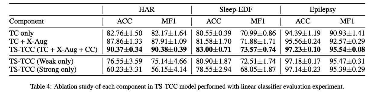
d) Ablation Study