(TF2) TS forecasting in TF

07. TS forecasting in TF

(참고) udemy - TF Developer in 2022

(1) TS forecasting & classification

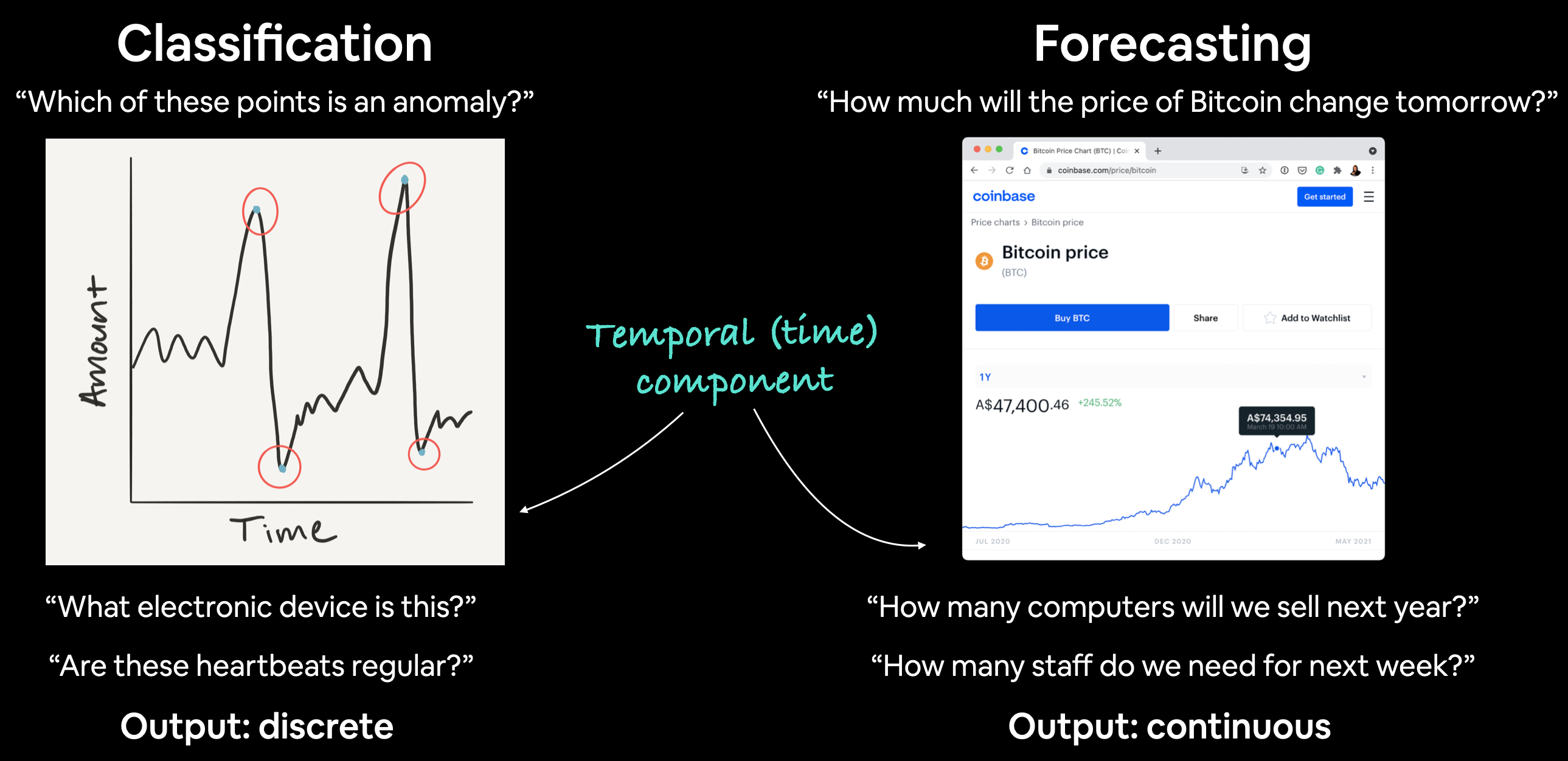
	Examples	Output
Classification	Anomaly detection, time series identification	Discrete
Forecasting	Predicting stock market prices, forecasting future demand for a product, stocking inventory requirements	Continuous

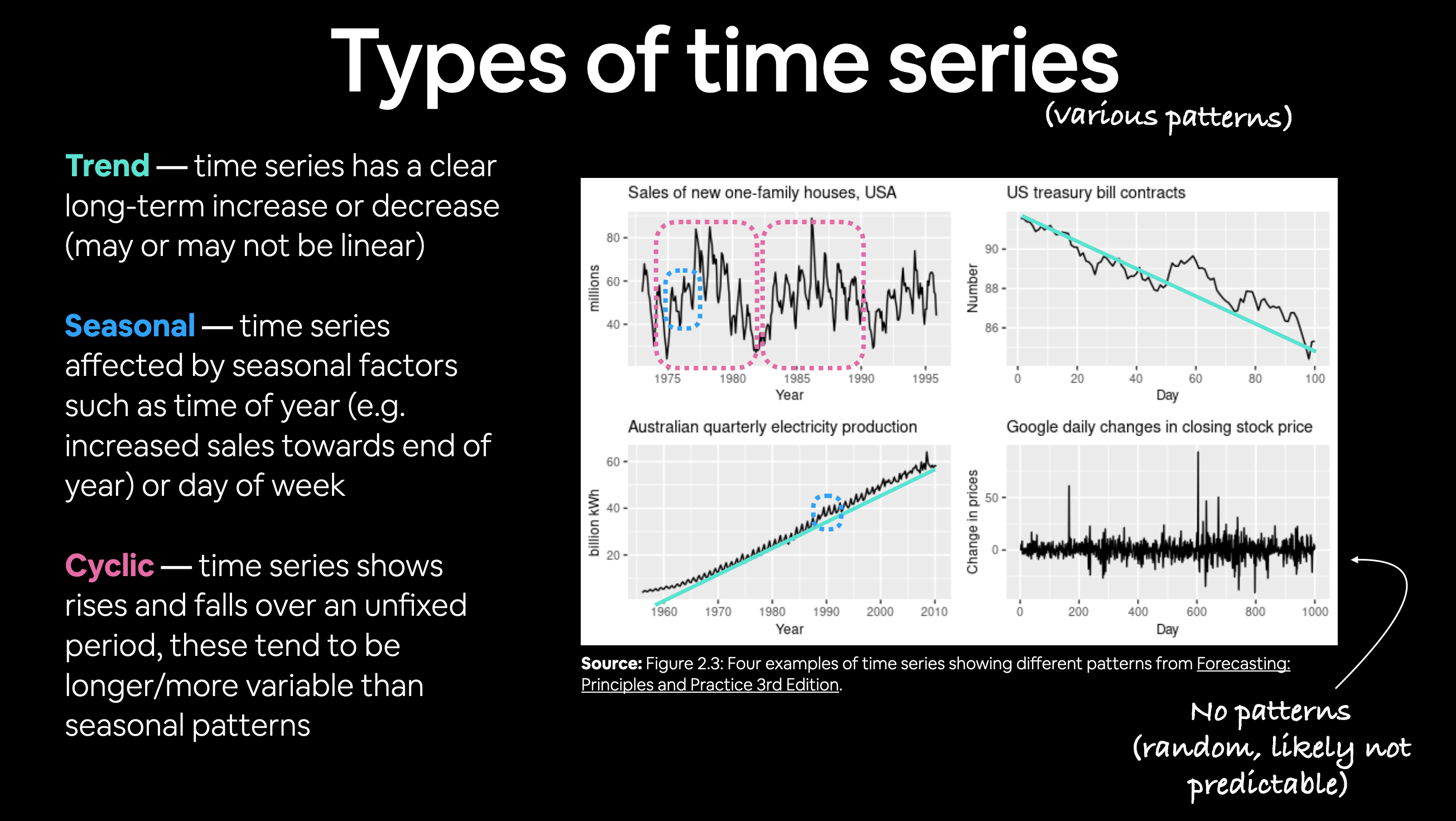
(2) Trend, Seasonality, Cycle

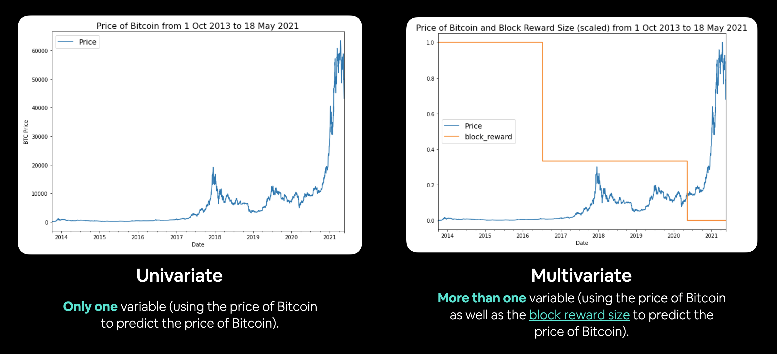
(3) Univariate vs Multivariate TS

(4) Train & Test split in TS

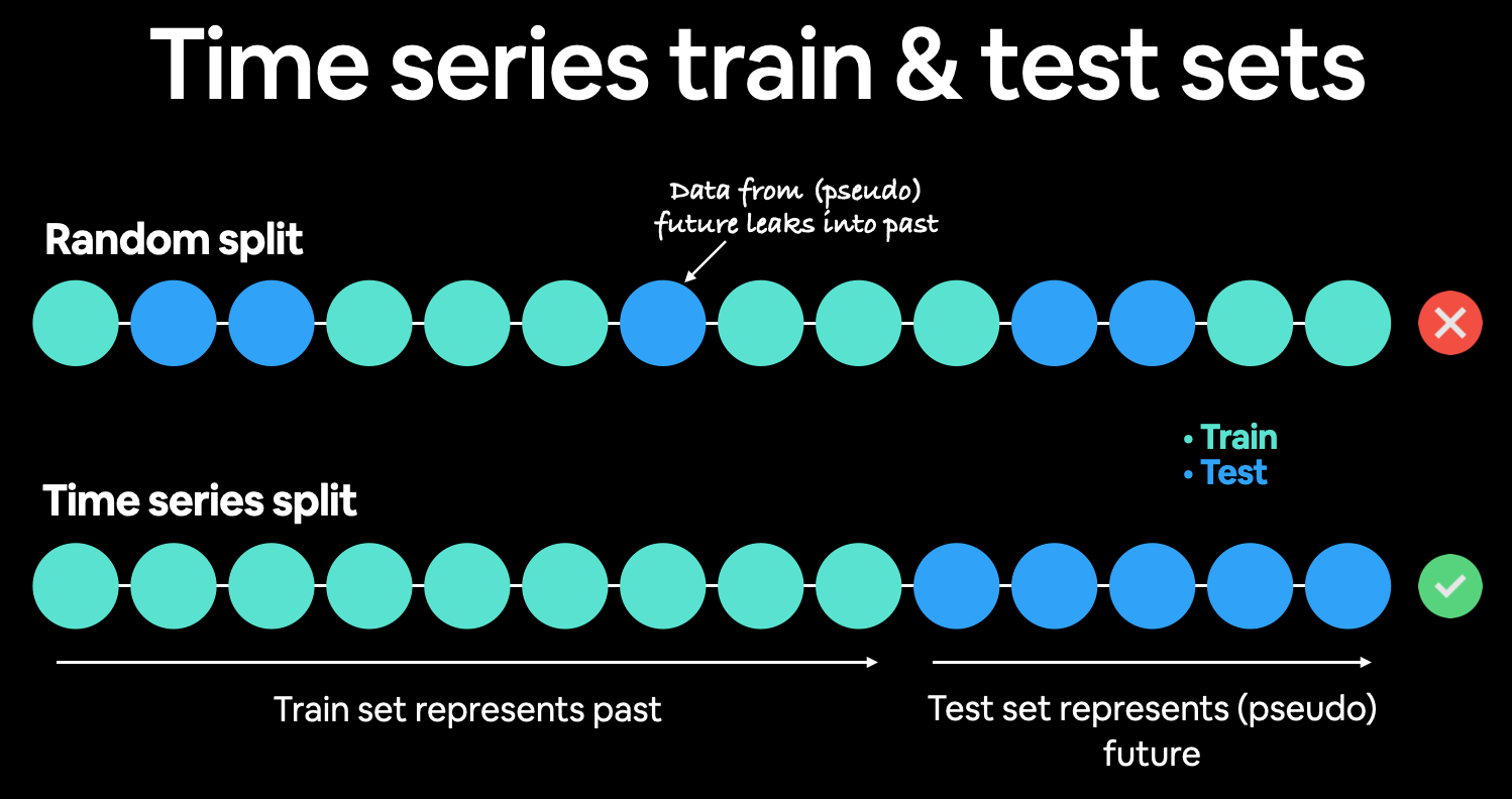
split_size = int(0.8 * len(prices)) 

X_train, y_train = timesteps[:split_size], prices[:split_size]
X_test, y_test = timesteps[split_size:], prices[split_size:]

(5) Evaluating TS models

a) scale-dependent errors

• MAE
  • tf.keras.metrics.mean_absolute_error()
• RMSE
  • tf.keras.metrics.mean_square_error()

b) percentage errors

• MAPE
  • tf.keras.metrics.mean_absolute_percentage_error()](https://www.tensorflow.org/api_docs/python/tf/keras/losses/MAPE)
• sMAPE
  • Recommended not to be used by Forecasting: Principles and Practice, though it is used in forecasting competitions.

c) scaled errors

• MASE

  • sktime’s mase_loss()

  • assuming no seasonality

  def mean_absolute_scaled_error(y_true, y_pred):
    mae = tf.reduce_mean(tf.abs(y_true - y_pred))
    mae_naive_no_season = tf.reduce_mean(tf.abs(y_true[1:] - y_true[:-1]))
    return mae / mae_naive_no_season
  

(6) Baseline models

Model/Library Name	Resource
Moving average	https://machinelearningmastery.com/moving-average-smoothing-for-time-series-forecasting-python/
ARIMA (Autoregression Integrated Moving Average)	https://machinelearningmastery.com/arima-for-time-series-forecasting-with-python/
sktime (Scikit-Learn for time series)	https://github.com/alan-turing-institute/sktime
TensorFlow Decision Forests (random forest, gradient boosting trees)	https://www.tensorflow.org/decision_forests
Facebook Kats (purpose-built forecasting and time series analysis library by Facebook)	https://github.com/facebookresearch/Kats
LinkedIn Greykite (flexible, intuitive and fast forecasts)	https://github.com/linkedin/greykite

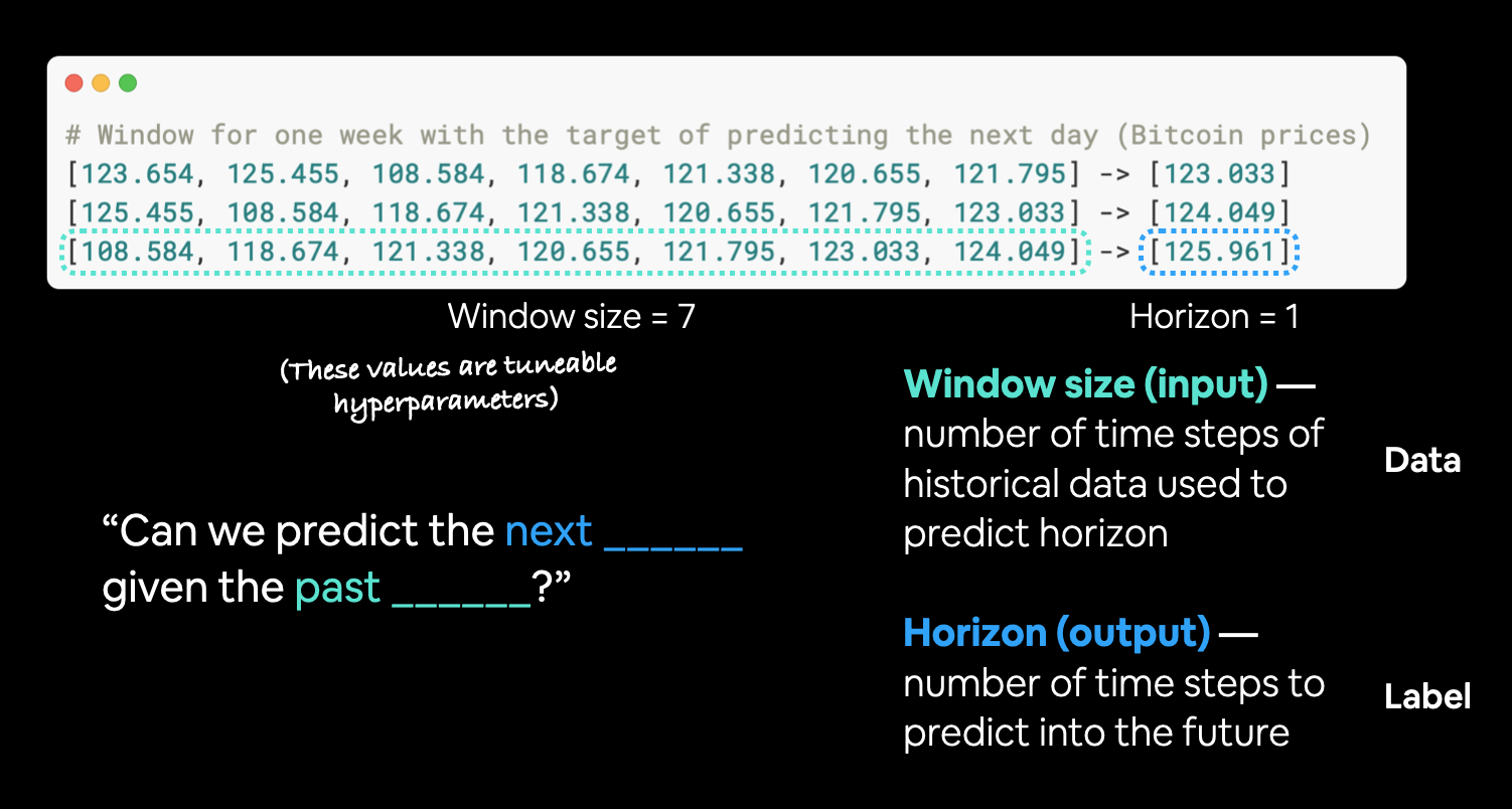
(7) Windowing Dataset

[0, 1, 2, 3, 4, 5, 6] -> [7]
[1, 2, 3, 4, 5, 6, 7] -> [8]
[2, 3, 4, 5, 6, 7, 8] -> [9]

(8) Checkpoint

import os

def create_model_checkpoint(model_name, save_path="model_experiments"):
  return tf.keras.callbacks.ModelCheckpoint(filepath=os.path.join(save_path, model_name),
                                            verbose=0, 
                                            save_best_only=True) 

(9) model 0 : naive forecast

가장 마지막 값을 예측값으로

naive_forecast = y_test[:-1] 

(10) model 1 : FC

Window = 7, Horizon = 1

HORIZON = 1

model_1 = tf.keras.Sequential([
  layers.Dense(128, activation="relu"),
  layers.Dense(HORIZON, activation="linear") ], 
  name="model_1_dense") 

Window = 30, Horizon = 7

HORIZON = 7

model_2 = tf.keras.Sequential([
  layers.Dense(128, activation="relu"),
  layers.Dense(HORIZON) ],
  name="model_2_dense")

(11) model 2 : Conv1D

• axis=1 (2번째 차원, channel 차원)에 1 넣어주기

model_4 = tf.keras.Sequential([
  layers.Lambda(lambda x: tf.expand_dims(x, axis=1)),
  layers.Conv1D(filters=128, kernel_size=5, padding="causal", activation="relu"),
  layers.Dense(HORIZON)], 
  name="model_4_conv1D")

(12) model 3 : RNN (LSTM)

inputs = layers.Input(shape=(WINDOW_SIZE))
#------------------------------------------------------------------------------------#
x = layers.Lambda(lambda x: tf.expand_dims(x, axis=1))(inputs) 
x = layers.LSTM(128, activation="relu")(x)
output = layers.Dense(HORIZON)(x)
#------------------------------------------------------------------------------------#
model_5 = tf.keras.Model(inputs=inputs, outputs=output, name="model_5_lstm")

(13) Ensembling results

def make_ensemble_preds(ensemble_models, data):
  ensemble_preds = []
  for model in ensemble_models:
    preds = model.predict(data)
    ensemble_preds.append(preds)
  return tf.constant(tf.squeeze(ensemble_preds))
  
ensemble_preds = make_ensemble_preds(ensemble_models=ensemble_models,
                                     data=test_dataset)

Prediction Interval

Prediction Intervals for Deep Learning Neural Networks

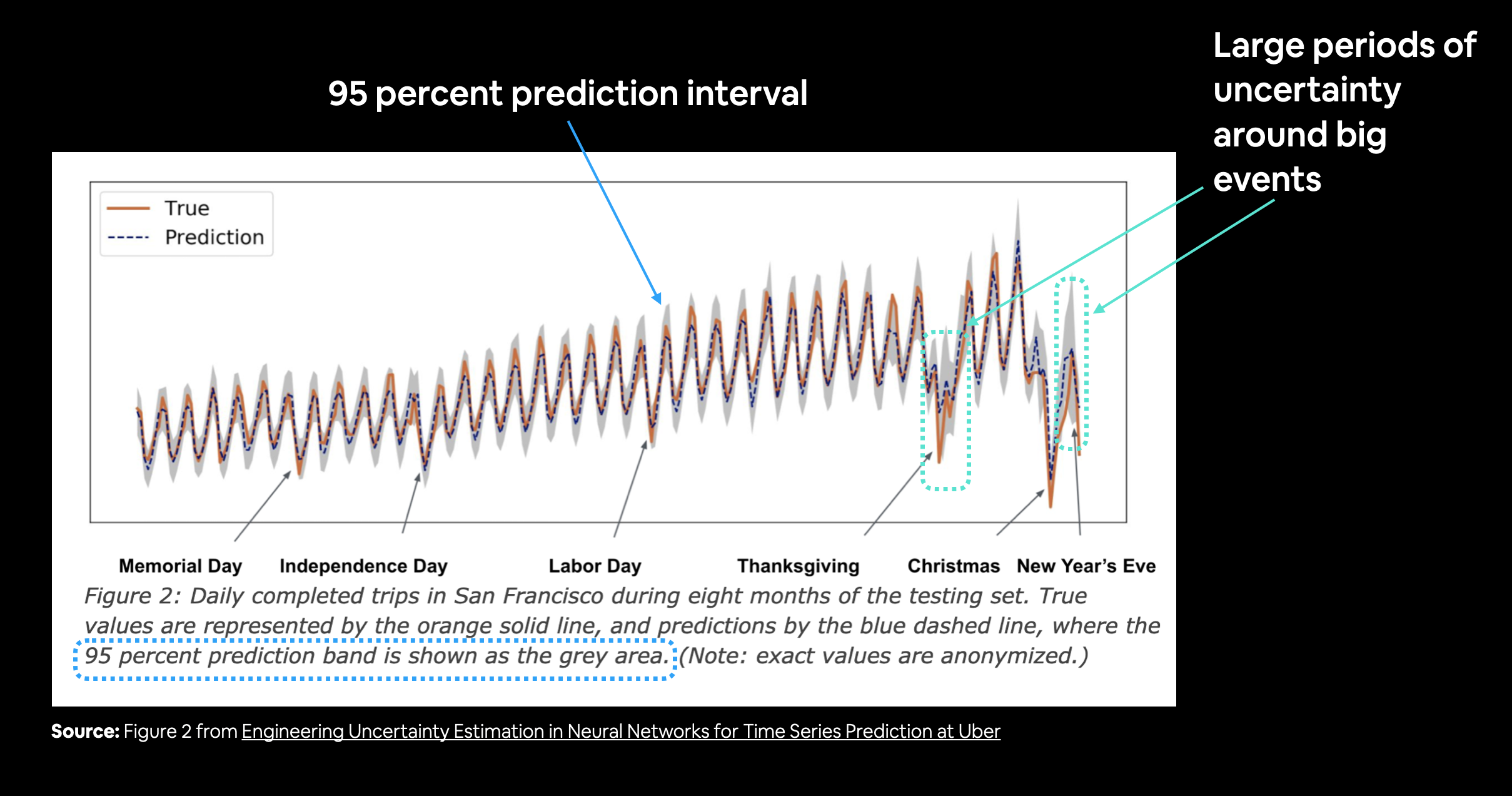
One way of getting the 95% condfidnece prediction intervals for a deep learning model is the bootstrap method:

1. Take the predictions from a number of randomly initialized models
2. Measure the standard deviation of the predictions
3. Multiply standard deviation by 1.96
   • (assuming the distribution is Gaussian, 95% of observations fall within 1.96 standard deviations of the mean, this is why we initialized our neural networks with a normal distribution)
4. To get the prediction interval upper and lower bounds, add and subtract the value obtained in (3) to the mean/median of the predictions made in (1)

def get_upper_lower(preds): 
  preds_mean = tf.reduce_mean(preds, axis=0)
  std = tf.math.reduce_std(preds, axis=0)
  interval = 1.96 * std 
  lower, upper = preds_mean - interval, preds_mean + interval
  return lower, upper

lower, upper = get_upper_lower(preds=ensemble_preds)

ensemble_median = np.median(ensemble_preds, axis=0)

offset=500
plt.figure(figsize=(10, 7))
plt.plot(X_test.index[offset:], y_test[offset:], "g", label="Test Data")
plt.plot(X_test.index[offset:], ensemble_median[offset:], "k-", label="Ensemble Median")
plt.xlabel("Date")
plt.ylabel("BTC Price")
plt.fill_between(X_test.index[offset:], 
                 (lower)[offset:], 
                 (upper)[offset:], label="Prediction Intervals")
plt.legend(loc="upper left", fontsize=14)