(paper) MAGNN ( Multi-Scale Adaptive GNN ) for MTS Forecasting

MAGNN ( Multi-Scale Adaptive GNN ) for MTS Forecasting (2022)

Contents

1. Abstract
2. Introduction
3. Related Works
   1. Graph Learning for MTS
4. Preliminaries
   1. Problem Formulation
   2. GNN
5. Methodology
   1. Framework
   2. Multi-scale Pyramid Network
   3. Adaptive Graph Learning
   4. Multi-scale Temporal GNN
   5. Scale-wise Fusion
   6. Output module & Objective function

0. Abstract

Backgound

• need to consider both complex intra-variable & inter-variable dependencies

• multi-scale temporal patterns in many real-world MTS

MAGNN

Multi-Scale Adaptive GNN

• Multi-scale pyramid network

  • preserve the underlying temporal dependencies at different time scale

• Adaptive graph learning module

  • to infer the scale specific inter-variable dependencies

• With (1) & (2)

  • (1) multi-scale feature representation
  • (2) scale-specific inter-variable dependencies

  use MAGNN to jointly model “inter” & “intra” variable dependencies

• Scale-wise fusion module

  • collaboration across different time scales
  • automatically capture the importance of contributed temporal patterns

1. Introduction

Exisiting works

(1) only consider temporal dependencies on a SINGLE time scale

• (reality) daily / weekly /monthly …

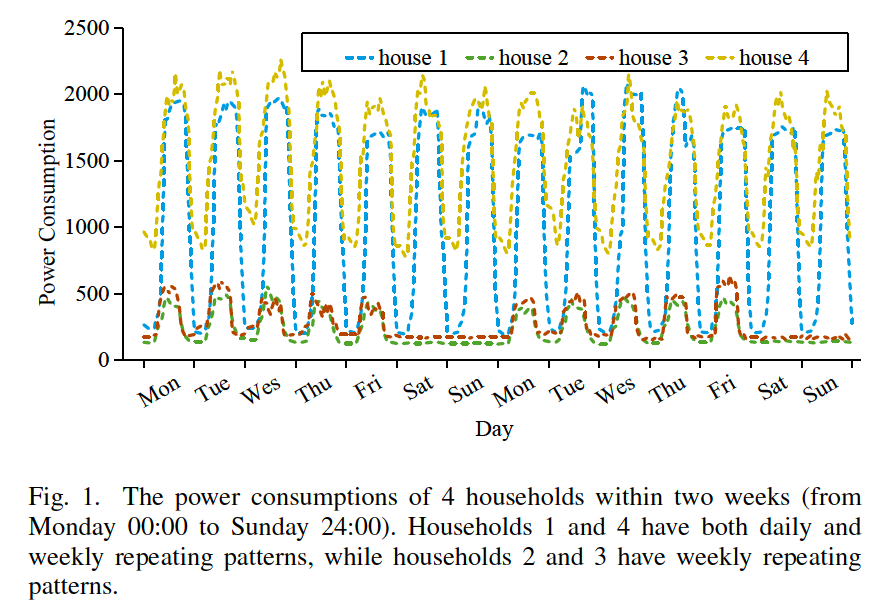
• ex) Power Consumption

  • mixture of SHORT & LONG term repeating patterns

    ( = multi-scale temporal patterns )

  

(2) learn a shared \(A\) matrix to reprsent rich inter-variable dependencies

• makes the models be BIASED to learn 1 type of prominent & shared temporal patterns

\(\rightarrow\) the complicated inter-variable dependencies need to be fully considered! ( when modeling multi-scale temporal patterns )

2. Related Works

(1) Graph Learning for MTS

Challenges of the GNNs-based MTS forecasting

• Obtaining a well-defined graph structure as the inter-variable dependencies
• solution (3 categories) :
  • prior-knowledge-based
  • rule-based
  • learning-based

a) Prior-knowledge based

use extra information ( ex. road networks / physical structures )

problem : require domain knowledge

b) Rule-based

provide data-driven manner to construct the graph structure

ex) causal discovery , entropy-based method, similarity based method

problem : non-parameterized methods \(\rightarrow\) limited flexibility,

( can only learn a kind of specific inter-variable dependency )

c) Learning-based

parameterized moudle to learn pairwise inter-variable

problem : existing works only learn “single inter-variable” dependencies

( make the models biased to learn one type of prominent and

shared temporal patterns among MTS )

3. Preliminaries

(1) Problem Formulation

Notation

• ts : \(\boldsymbol{X}=\left\{\boldsymbol{x}_{1}, \boldsymbol{x}_{2}, \ldots, \boldsymbol{x}_{t}, \ldots, \boldsymbol{x}_{T}\right\}\)
  • \(\boldsymbol{X} \in \mathbb{R}^{N \times T}\).
  • \(\boldsymbol{x}_{t} \in \mathbb{R}^{N}\).
• predict \(\widehat{\boldsymbol{x}}_{T+h} \in \mathbb{R}^{N}\)
• model : \(\widehat{\boldsymbol{x}}_{T+h}=\mathcal{F}\left(\boldsymbol{x}_{1}, \boldsymbol{x}_{2}, \ldots, \boldsymbol{x}_{T} ; \theta\right)\)

Graph \((V, E)\)

• number of nodes : \(N\)
• \(i\)th node : \(v_{i} \in V\)
  • \(\left\{\boldsymbol{x}_{1, i}, \boldsymbol{x}_{2, i}, \ldots, \boldsymbol{x}_{T, i}\right\}\).

• Edge : \(\left(v_{i}, v_{j}\right) \in E\)

• model : \(\widehat{\boldsymbol{x}}_{T+h}=\mathcal{F}\left(\boldsymbol{x}_{1}, \boldsymbol{x}_{2}, \ldots, \boldsymbol{x}_{T} ; G ; \theta\right) .\)

Weighted Adjacency matrix \(\boldsymbol{A} \in \mathbb{R}^{N \times N}\)

• \(\boldsymbol{A}_{i, j}>0\) if \(\left(v_{i}, v_{j}\right) \in E\)
• \(\boldsymbol{A}_{i, j}=0\) if \(\left(v_{i}, v_{j}\right) \notin E\)

(2) GNN

GCN operation :

• \(\boldsymbol{x} *_{G} \theta=\sigma\left(\theta\left(\widetilde{\boldsymbol{D}}^{-\frac{1}{2}} \widetilde{\boldsymbol{A}} \widetilde{\boldsymbol{D}}^{-\frac{1}{2}}\right) \boldsymbol{x}\right)\).
  • \(\widetilde{\boldsymbol{A}}=\boldsymbol{I}_{n}+\boldsymbol{A}\).
  • \(\widetilde{\boldsymbol{D}}_{i i}=\sum_{j} \widetilde{\boldsymbol{A}}_{i j}\).

by stacking GCN operations…can aggregate info of multi-order neighbors

4. Methodology

(1) Framework

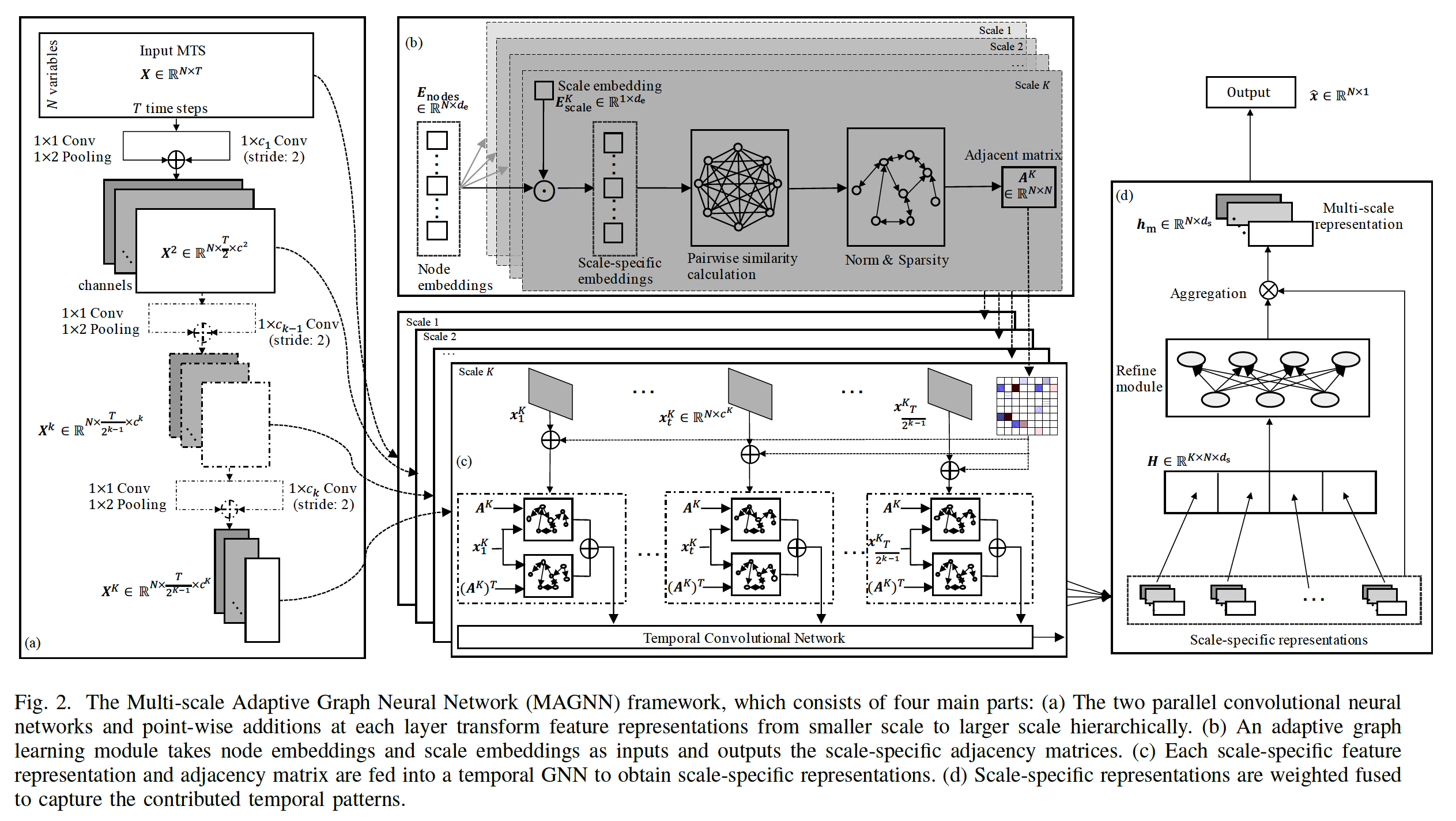
4 main parts

1. Multi-scale pyramid networrk
2. Adaptive Graph Learning module
   • to automatically infer inter-variable dependencies
3. Multi-scale temporal GNN
   • to capture all kinds of scale-specific temporal patterns
4. Scale-wise fusion module
   • to effectively promote the collaboration across different scale

(2) Multi-scale Pyramid Network

to preserve the underlying temporal dependencies at different time scales

• small scale : more fine-grained details
• large scale : slow-varying trends

generates multi-scale feature representations ( from each layer )

Input : \(\boldsymbol{X} \in \mathbb{R}^{N \times T}\)

Output : feature representations of \(K\) scales

• \(k\) th scale : \(\boldsymbol{X}^{k} \in \mathbb{R}^{N \times \frac{T}{2^{k-1}} \times c^{k}}\)
  • \(\frac{T}{2^{k-1}}\) : sequence length
  • \(c^{k}\) : channel size

Model :

• use CNN to capture local patterns
• different filter size in different layer
  • beginning layer : LARGE filter
  • end layer : SMALL filter
• stride size of convolution is set to 2 to increase the time scale

Details : \(\boldsymbol{X}^{k}=\boldsymbol{X}_{\text {rec }}^{k}+\boldsymbol{X}_{\text {norm }}^{k}\)

• (1) \(\boldsymbol{X}_{\mathrm{rec}}^{k}=\operatorname{ReLU}\left(\boldsymbol{W}_{\mathrm{rec}}^{k} \otimes \boldsymbol{X}^{k-1}+\boldsymbol{b}_{\mathrm{rec}}^{k}\right)\)
  • using only 1 CNN … not flexible!
• (2) \(\boldsymbol{X}_{\mathrm{norm}}^{k}=\operatorname{Pooling}\left(\operatorname{ReLU}\left(\boldsymbol{W}_{\mathrm{norm}}^{k} \otimes \boldsymbol{X}^{k-1}+\boldsymbol{b}_{\mathrm{norm}}^{k}\right)\right)\)
  • use 1 more (parallel) CNN ( kernel size 1x1 & 1x2 pooling layer )

Summary : the learned multi-scale feature representations are flexible and comprehensive to preserve various kinds of temporal dependencies

( to avoid the interaction between the variables of MTS, the convolutional operations are performed on the time dimension )

(3) Adaptive Graph Learning

Automatically generates \(A\) matrix

• existing methods ) only learrns SHARED \(A\)
• essential to learn MULTIPLE SCALE-SPECIFIC \(A\)

But, directly learning a unique \(A\) … to costly! ( too many parameters )

\(\rightarrow\) propose a AGL (Adaptive Graph Learning) module!

AGL initializes 2 parameters

• (1) shared node embeddings : \(\boldsymbol{E}_{\text {nodes }} \in \mathbb{R}^{N \times d_{\mathrm{e}}}\)
  • SAME across all scales & \(d_{\mathrm{e}} \ll N ; 2\)
• (2) scale embeddings : \(\boldsymbol{E}_{\text {scale }} \in \mathbb{R}^{K \times d_{e}}\)
  • DIFFERENT across all scales

AGL module includes…

• (1) shared node embeddings
• (2) \(K\) scale-specific layers

Procedure

• step 1) \(\boldsymbol{E}_{\text {nodes }}\) are randomly initialized

• step 2) \(\boldsymbol{E}_{\text {nodes }}\) are fed into scale-specific layer

  • ( for \(k^{th}\) layer ) \(\boldsymbol{E}_{\text {scale }}^{k} \in \mathbb{R}^{1 \times d_{e}}\) are randomly initiailized

  • then, \(\boldsymbol{E}_{\text {spec }}^{k}=\boldsymbol{E}_{\text {nodes }} \odot \boldsymbol{E}_{\text {scale }}^{k}\), where \(\boldsymbol{E}_{\text {spec }}^{k} \in \mathbb{R}^{N \times d_{\mathrm{e}}}\)

    • \(\boldsymbol{E}_{\text {spec }}^{k}\) : scale-specific embedding in \(k^{th}\) layer

      ( contains both node & scale-spcific information )

• step 3) calculate pairwise node similarities

  • \(\begin{aligned} \boldsymbol{M}_{1}^{k} &=\left[\tanh \left(\boldsymbol{E}_{\mathrm{spec}}^{k} \theta^{k}\right)\right]^{T} \\ \boldsymbol{M}_{2}^{k} &=\tanh \left(\boldsymbol{E}_{\mathrm{spec}}^{k} \varphi^{k}\right) \\ \boldsymbol{A}_{\text {full }}^{k} &=\operatorname{Re} L U\left(\boldsymbol{M}_{1}^{k} \boldsymbol{M}_{2}^{k}-\left(\boldsymbol{M}_{2}^{k}\right)^{T}\left(\boldsymbol{M}_{1}^{k}\right)^{T}\right) \end{aligned}\).
  • \(\boldsymbol{A}_{\text {full }}^{k} \in \mathbb{R}^{N \times N}\) are then normalized to \(0-1\)

• step 4) make adjacency matrix SPARSE

  • \(\boldsymbol{A}^{k}=\operatorname{Sparse}\left(\operatorname{Softmax}\left(\boldsymbol{A}_{\text {full }}^{k}\right)\right)\).
  • Sparse function :
    • \(\boldsymbol{A}_{i j}^{k}=\left\{\begin{array}{ll} \boldsymbol{A}_{i j}^{k}, & \boldsymbol{A}_{i j}^{k} \in \operatorname{Top} K\left(\boldsymbol{A}_{i *}^{k}, \tau\right) \\ 0, & \boldsymbol{A}_{i j}^{k} \notin \operatorname{Top} K\left(\boldsymbol{A}_{i *}^{k}, \tau\right) \end{array}\right.\).

• step 5) get SCALE-SPECIFIC \(A\)

  • \(\left\{\boldsymbol{A}^{1}, \ldots, \boldsymbol{A}^{k}, \ldots, \boldsymbol{A}^{K}\right\}\).

(4) Multi-scale Temporal GNN

2 inputs

• (1) \(\left\{\boldsymbol{X}^{1}, \ldots, \boldsymbol{X}^{k}, \ldots, \boldsymbol{X}^{K}\right\}\) ( from multi-scale pyramid network)
• (2) \(\left\{\boldsymbol{A}^{1}, \ldots, \boldsymbol{A}^{k}, \ldots, \boldsymbol{A}^{K}\right\}\) ( from AGL module )

MTG (Multi-scale Temporal GNN)

• capture scale-specific temporal patterns across time steps & variables

Existing works

• GRU + GNN : gradient vanishing/exploding
• TCNs : very good!

\(\rightarrow\) combine GNN & TCNs ( insead of GRU )

details of MTG

• \(K\) temporal GNN ( TCN + GNN )

• for \(k^{th}\) scale, split \(\mathbf{X}^{k}\) at time dimension

  \(\rightarrow\) obtain \(\left\{\boldsymbol{x}_{1}^{k}, \ldots, \boldsymbol{x}_{t}^{k}, \ldots, \boldsymbol{x}_{\frac{T}{2 k-1}}^{k}\right\}\left(\boldsymbol{x}_{t}^{k} \in \mathbb{R}^{N \times c^{k}}\right)\)

• use 2 GNNs, to capture both IN & OUT coming information

  • \(\widetilde{\boldsymbol{h}}_{t}^{k}=G N N_{\mathrm{in}}^{k}\left(\boldsymbol{x}_{t}^{k}, \boldsymbol{A}^{k}, \boldsymbol{W}_{\mathrm{in}}^{k}\right)+G N N_{\mathrm{out}}^{k}\left(\boldsymbol{x}_{t}^{k},\left(\boldsymbol{A}^{k}\right)^{T}, \boldsymbol{W}_{\mathrm{out}}^{k}\right)\).

• then, obtain \(\left\{\widetilde{\boldsymbol{h}}_{1}^{k}, \ldots, \widetilde{\boldsymbol{h}}_{t}^{k}, \ldots, \widetilde{\boldsymbol{h}}_{\frac{T}{2^{k}}}^{k}\right\}\)

  \(\rightarrow\) fed into TCN & obtain \(\tilde{\mathbf{h}}\)

  \(\boldsymbol{h}^{k}=\operatorname{TCN} N^{k}\left(\left[\widetilde{\boldsymbol{h}}_{1}^{k}, \ldots, \widetilde{\boldsymbol{h}}_{t}^{k}, \ldots, \widetilde{\boldsymbol{h}}_{\frac{T}{2^{k}}}^{k}\right], \boldsymbol{W}_{\mathrm{tcn}}^{k}\right)\).

Advantages of using MTG

• (1) capture SCALE-SPECIFIC temporal patterns
• (2) GCN operators enables the model to consider INTER-variable dependencies

(5) Scale-wise Fusion

Input : scale-specific representations

• \(\left\{\boldsymbol{h}^{1}, \ldots, \boldsymbol{h}^{k}, \ldots, \boldsymbol{h}^{K}\right\}\), where \(\boldsymbol{h}^{k} \in \mathbb{R}^{N \times d_{\mathrm{s}}}\)
  • \(d_{\mathrm{s}}\) : output dimension of TCN

Intuitive solution : concatenate them / global pooling

\(\rightarrow\) problem : treats them equally!

\(\rightarrow\) propose a scalewise fusion module

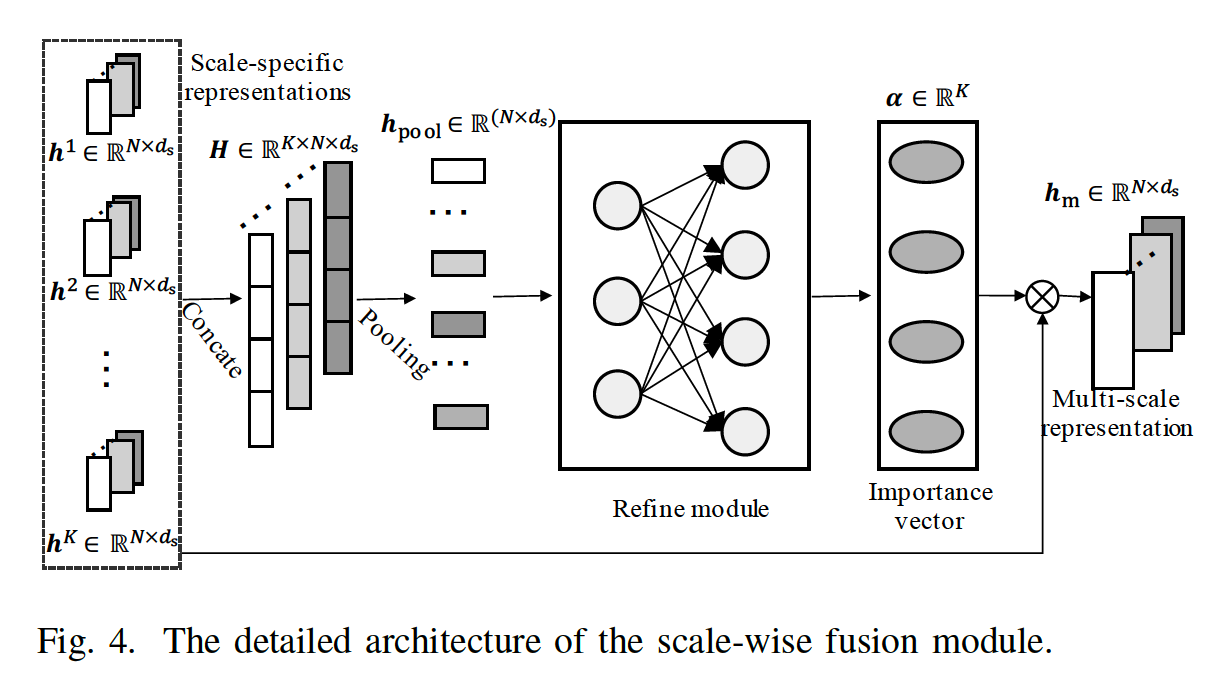
Details

• step 1) concatenate

  • \(\boldsymbol{H}=\operatorname{Concat}\left(\boldsymbol{h}^{1}, \ldots, \boldsymbol{h}^{k}, \ldots, \boldsymbol{h}^{K}\right)\)….\(\boldsymbol{H} \in \mathbb{R}^{K \times N \times d_{s}}\)

• step 2) average pooling ( on scale dimension)

  • \(\boldsymbol{h}_{\mathrm{pool}}=\frac{\sum_{k=1}^{K} \boldsymbol{H}^{k}}{K}\)………. \(h_{\text {pool }} \in \mathbb{R}^{1 \times N \times d_{\mathrm{s}}}\)

• step 3) flatten

• step 4) fed into refining module

  • \(\begin{aligned} &\boldsymbol{\alpha}_{1}=\operatorname{ReLU}\left(\boldsymbol{W}_{1} \boldsymbol{h}_{\mathrm{pool}}+\boldsymbol{b}_{1}\right) \\ &\boldsymbol{\alpha}=\operatorname{Sigmoid}\left(\boldsymbol{W}_{2} \boldsymbol{\alpha}_{1}+\boldsymbol{b}_{2}\right) \end{aligned}\).

    ( = importance score ( importance of scale-specific representation ) )

• step 5) weighted average & ReLU

  • \(\boldsymbol{h}_{\mathrm{m}}=\operatorname{ReLU}\left(\sum_{k=1}^{K} \boldsymbol{\alpha}[k] \times \boldsymbol{h}^{k}\right)\).

    ( = final multi-scale representation)

(6) Output Module & Objective function

Output layer : 1\(\times d_s\) CNN & \(1\times1\) CNN

• Input : \(\boldsymbol{h}_{\mathrm{m}} \in \mathbb{R}^{N \times d_{\mathrm{s}}}\)

• Output : \(\widehat{\boldsymbol{x}} \in \mathbb{R}^{N \times 1}\)

Loss Function : \(\mathcal{L}_{2}=\frac{1}{\mathcal{T}_{\text {train }}} \sum_{i=1}^{\mathcal{T}_{\text {rain }}} \sum_{j=1}^{N}\left(\widehat{\boldsymbol{x}}_{i, j}-\boldsymbol{x}_{i, j}\right)^{2}\).