(paper 91) Autoregressive Denoising Diffusion Models for Multivariate Probabilistic Time Series Forecasting

Autoregressive Denoising Diffusion Models for Multivariate Probabilistic Time Series Forecasting

Contents

1. Abstract
2. Introduuction
3. Diffusion Probabilistic Model
4. TimeGrad
   1. Training
   2. Inference
   3. Scaling
5. Experiments
   1. Evaluation Metric and Dataset

0. Abstract

TimeGrad

• AR model for MTS probabilistic forecasting
  • samples from the data distribution at each time step by estimating its gradient.
• Diffusion probabilistic models
• Learns gradients by optimizing a variational bound on the data likelihood

1. Introduction

TimeGrad = Autoregressive EBMs

• to solve the MTS probabilistic forecasting problem
• train a model with all the inductive biases of probabilistic TS forecasting

Autoregressive-EBM

• AR) Good performance in extrapolation into the future
• EBM) Flexibility of EBMs as a general purpose high-dimensional distribution model

Setup

• Section 2) Notation & Detail of EBM
• Section 3) MTS probabilsitic problem & TimeGrad
• Section 4) Experiments

2. Diffusion Probabilistic Model

Notation

• \(\mathbf{x}^0 \sim q_{\mathcal{X}}\left(\mathbf{x}^0\right)\) : Multivariate training vector

  • input space \(\mathcal{X}=\mathbb{R}^D\)

• \(p_\theta\left(\mathbf{x}^0\right)\) : PDF which aims to approximate \(q_{\mathcal{X}}\left(\mathbf{x}^0\right)\)

  ( + allows for easy sampling )

Diffusion models

\(p_\theta\left(\mathbf{x}^0\right):=\int p_\theta\left(\mathbf{x}^{0: N}\right) \mathrm{d} \mathbf{x}^{1: N}\),

• where \(\mathbf{x}^1, \ldots, \mathbf{x}^N\) are latents of dimension \(\mathbb{R}^D\).

a) Forward Process ( = Add Noise )

Unlike VAE, approximate posterior \(q\left(\mathbf{x}^{1: N} \mid \mathbf{x}^0\right)\) is not trainable!

But fixed to ”Markov chain”

\(q\left(\mathbf{x}^{1: N} \mid \mathbf{x}^0\right)=\Pi_{n=1}^N q\left(\mathbf{x}^n \mid \mathbf{x}^{n-1}\right)\).

• \(q\left(\mathbf{x}^n \mid \mathbf{x}^{n-1}\right):=\mathcal{N}\left(\mathbf{x}^n ; \sqrt{1-\beta_n} \mathbf{x}^{n-1}, \beta_n \mathbf{I}\right)\).
• increasing variance schedule \(\beta_1, \ldots, \beta_N\) with \(\beta_n \in(0,1)\).

Summary

\(q\left(\mathbf{x}^n \mid \mathbf{x}^0\right)=\mathcal{N}\left(\mathbf{x}^n ; \sqrt{\bar{\alpha}_n} \mathbf{x}^0,\left(1-\bar{\alpha}_n\right) \mathbf{I}\right)\).

• \(\alpha_n:=1-\beta_n\).
• \(\bar{\alpha}_n:=\Pi_{i=1}^n \alpha_i\).

\(q\left(\mathbf{x}^{n-1} \mid \mathbf{x}^n, \mathbf{x}^0\right)\) are tractable given by

• \(q\left(\mathbf{x}^{n-1} \mid \mathbf{x}^n, \mathbf{x}^0\right)=\mathcal{N}\left(\mathbf{x}^{n-1} ; \tilde{\mu}_n\left(\mathbf{x}^n, \mathbf{x}^0\right), \tilde{\beta}_n \mathbf{I}\right)\).
  • \(\tilde{\mu}_n\left(\mathbf{x}^n, \mathbf{x}^0\right):=\frac{\sqrt{\bar{\alpha}_{n-1}} \beta_n}{1-\bar{\alpha}_n} \mathbf{x}^0+\frac{\sqrt{\alpha_n}\left(1-\bar{\alpha}_{n-1}\right)}{1-\bar{\alpha}_n} \mathbf{x}^n\).
  • \(\tilde{\beta}_n:=\frac{1-\bar{\alpha}_{n-1}}{1-\bar{\alpha}_n} \beta_n\).

b) Reverse Process ( = Remove Noise )

Model joint distn \(p_\theta\left(\mathbf{x}^{0: N}\right)\)

Also defined as a “Markov chain”

• with learned Gaussian transitions starting with \(p\left(\mathbf{x}^N\right)=\mathcal{N}\left(\mathbf{x}^N ; \mathbf{0}, \mathbf{I}\right)\)

\(p_\theta\left(\mathbf{x}^{0: N}\right):=p\left(\mathbf{x}^N\right) \Pi_{n=N}^1 p_\theta\left(\mathbf{x}^{n-1} \mid \mathbf{x}^n\right)\).

• \(p_\theta\left(\mathbf{x}^{n-1} \mid \mathbf{x}^n\right):=\mathcal{N}\left(\mathbf{x}^{n-1} ; \mu_\theta\left(\mathbf{x}^n, n\right), \Sigma_\theta\left(\mathbf{x}^n, n\right) \mathbf{I}\right)\).

Both \(\mu_\theta: \mathbb{R}^D \times \mathbb{N} \rightarrow \mathbb{R}^D\) and \(\Sigma_\theta: \mathbb{R}^D \times \mathbb{N} \rightarrow \mathbb{R}^{+}\)take two inputs

• (1) Variable \(\mathbf{x}^n \in \mathbb{R}^D\)
• (2) Noise index \(n \in \mathbb{N}\).

Goal of \(p_\theta\left(\mathbf{x}^{n-1} \mid \mathbf{x}^n\right)\)

= eliminate the Gaussian noise added

= \(\theta\) are learned to fit the data distribution \(q_{\mathcal{X}}\left(\mathbf{x}^0\right)\)

• by minimizing the NLL via a variational bound

(1) \(\begin{array}{r} \min _\theta \mathbb{E}_{q\left(\mathbf{x}^0\right)}\left[-\log p_\theta\left(\mathbf{x}^0\right)\right] \leq \min _\theta \mathbb{E}_{q\left(\mathbf{x}^{0: N}\right)}\left[-\log p_\theta\left(\mathbf{x}^{0: N}\right)+\log q\left(\mathbf{x}^{1: N} \mid \mathbf{x}^0\right)\right] \end{array}\).

Backward Process in detail

The upper bound is equal to …

(2) \(\min _\theta \mathbb{E}_{q\left(\mathbf{x}^{0: N}\right)}\left[-\log p\left(\mathbf{x}^N\right)-\sum_{n=1}^N \log \frac{p_\theta\left(\mathbf{x}^{n-1} \mid \mathbf{x}^n\right)}{q\left(\mathbf{x}^n \mid \mathbf{x}^{n-1}\right)}\right]\).

The above objective can be written as …

KL-divergence btw Gaussian

(3) \(-\log p_\theta\left(\mathbf{x}^0 \mid \mathbf{x}^1\right)+D_{\mathrm{KL}}\left(q\left(\mathbf{x}^N \mid \mathbf{x}^0\right) \mid p\left(\mathbf{x}^N\right)\right) +\sum_{n=2}^N D_{\mathrm{KL}}\left(q\left(\mathbf{x}^{n-1} \mid \mathbf{x}^n, \mathbf{x}^0\right) \mid p_\theta\left(\mathbf{x}^{n-1} \mid \mathbf{x}^n\right)\right)\).

• \(\begin{aligned} D_{\mathrm{KL}}( & \left.\left(\mathbf{x}^{n-1} \mid \mathbf{x}^n, \mathbf{x}^0\right) \mid p_\theta\left(\mathbf{x}^{n-1} \mid \mathbf{x}^n\right)\right)= \mathbb{E}_q\left[\frac{1}{2 \Sigma_\theta} \mid \mid \tilde{\mu}_n\left(\mathbf{x}^n, \mathbf{x}^0\right)-\mu_\theta\left(\mathbf{x}^n, n\right) \mid \mid ^2\right]+C \end{aligned}\).

Instead of a parametrization of \(p_\theta\) that predicts \(\tilde{\mu}\)

Write \(\mathbf{x}^n\left(\mathbf{x}^0, \epsilon\right)=\sqrt{\bar{\alpha}_n} \mathbf{x}^0+\) \(\sqrt{1-\bar{\alpha}_n} \epsilon\) for \(\epsilon \sim \mathcal{N}(\mathbf{0}, \mathbf{I})\)

\(\rightarrow\) Then the formula for \(\tilde{\mu}\) to obtain that \(\mu_\theta\) must predict \(\left(\mathbf{x}^n-\beta_n \epsilon / \sqrt{1-\bar{\alpha}_n}\right) / \sqrt{\alpha_n}\),

\(\mu_\theta\left(\mathbf{x}^n, n\right)=\frac{1}{\sqrt{\alpha_n}}\left(\mathbf{x}^n-\frac{\beta_n}{\sqrt{1-\bar{\alpha}_n}} \epsilon_\theta\left(\mathbf{x}^n, n\right)\right)\).

• where \(\epsilon_\theta\) is a network which predicts \(\epsilon \sim \mathcal{N}(\mathbf{0}, \mathbf{I})\) from \(\mathbf{x}^n\)

Result : objective simplifies to …

\(\mathbb{E}_{\mathbf{x}^0, \epsilon}\left[\frac{\beta_n^2}{2 \Sigma_\theta \alpha_n\left(1-\bar{\alpha}_n\right)} \mid \mid \epsilon-\epsilon_\theta\left(\sqrt{\bar{\alpha}_n} \mathbf{x}^0+\sqrt{1-\bar{\alpha}_n} \epsilon, n\right) \mid \mid ^2\right]\).

Sampling from the reverse process

Reverse process \(\mathbf{x}^{n-1} \sim\) \(p_\theta\left(\mathbf{x}^{n-1} \mid \mathbf{x}^n\right)\)

• \(\mathbf{x}^{n-1}=\frac{1}{\sqrt{\alpha_n}}\left(\mathbf{x}^n-\frac{\beta_n}{\sqrt{1-\bar{\alpha}_n}} \epsilon_\theta\left(\mathbf{x}^n, n\right)\right)+\sqrt{\Sigma_\theta} \mathbf{z}\).
  • where \(\mathbf{z} \sim \mathcal{N}(\mathbf{0}, \mathbf{I})\) for \(n=N, \ldots, 2\) and \(\mathbf{z}=\mathbf{0}\) when \(n=1\).

3. TimeGrad

Notation

• entities of MTS : \(x_{i, t}^0 \in\) \(\mathbb{R}\) for \(i \in\{1, \ldots, D\}\)
• MTS vector at time \(t\) : \(\mathbf{x}_t^0 \in \mathbb{R}^D\).

Task : predict MTS distribution

• split this contiguous sequence into …
  • (1) context window of size \(\left[1, t_0\right)\)
  • (2) prediction interval \(\left[t_0, T\right]\),

DeepAR

• Univariate probabilistic forecasting model
• Maximize log-likelihood of each entity \(x_{i, t}^0\) at a time step \(t \in\left[t_0, T\right]\)
• This is done with respect to the parameters of some chosen distributional model via the state of an RNN derived from its previous time step \(x_{i, t-1}^0\) and its corresponding covariates \(\mathbf{c}_{i, t-1}\).
  • The emission distribution model, which is typically Gaussian for real-valued data or negative binomial for count data, is selected to best match the statistics of the time series and the network incorporates activation functions that satisfy the constraints of the distribution’s parameters, e.g. a softplus () for the scale parameter of the Gaussian.

Straightforawrd way to deal with MTS?

• use a factorizing output distribution instead

• Full joint distribution

  • ex) Multivariate Gaussian

    \(\rightarrow\) the full covariance matrix …. impractical ( \(O(D^3)\) )

TimeGrad

Learn a model of the conditional distribution of the future time steps of a MTS

• given its past and covariates

\(q_{\mathcal{X}}\left(\mathbf{x}_{t_0: T}^0 \mid \mathbf{x}_{1: t_0-1}^0, \mathbf{c}_{1: T}\right)=\Pi_{t=t_0}^T q_{\mathcal{X}}\left(\mathbf{x}_t^0 \mid \mathbf{x}_{1: t-1}^0, \mathbf{c}_{1: T}\right)\).

Assumption

• the covariates are known for all the time points
• and each factor is learned via a conditional denoising diffusion model

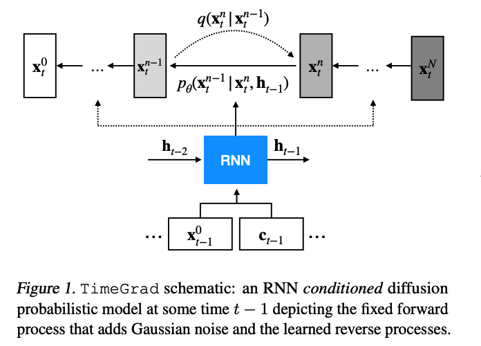
To model the temporal dynamics, use RNN architecture we employ the autoregressive recurrent

• \(\mathbf{h}_t=\operatorname{RNN}_\theta\left(\operatorname{concat}\left(\mathbf{x}_t^0, \mathbf{c}_t\right), \mathbf{h}_{t-1}\right)\).

Thus we can approximate the above as…

• \(\Pi_{t=t_0}^T p_\theta\left(\mathbf{x}_t^0 \mid \mathbf{h}_{t-1}\right)\).

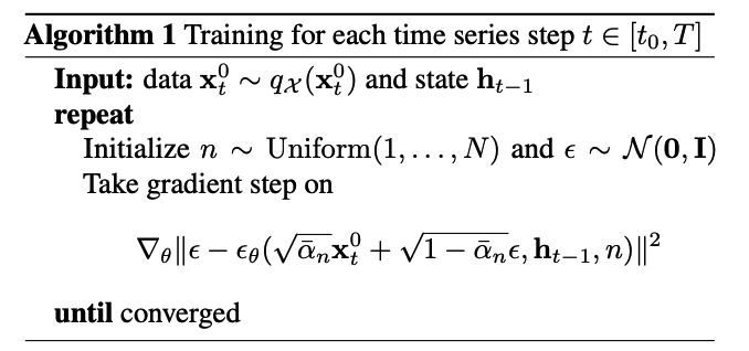
(1) Training

Randomly sampling context & adjoining prediction sized windows

Optimizing the parameters \(\theta\) that minimize NLL

• \(\sum_{t=t_0}^T-\log p_\theta\left(\mathbf{x}_t^0 \mid \mathbf{h}_{t-1}\right)\).

Objective Function :

• \(\mathbb{E}_{\mathbf{x}_t^0, \epsilon, n}\left[ \mid \mid \epsilon-\epsilon_\theta\left(\sqrt{\bar{\alpha}_n} \mathbf{x}_t^0+\sqrt{1-\bar{\alpha}_n} \epsilon, \mathbf{h}_{t-1}, n\right) \mid \mid ^2\right]\).

• when we choose the variance to be \(\Sigma_\theta=\tilde{\beta}_n\)
• \(\epsilon_\theta\) network : also conditioned on the hidden state

(2) Inference

Step 1) Run the RNN over the last context sized window

• obtain the hidden state \(\mathbf{h}_T\)

Step 2) Sampling procedure in Algorithm 2

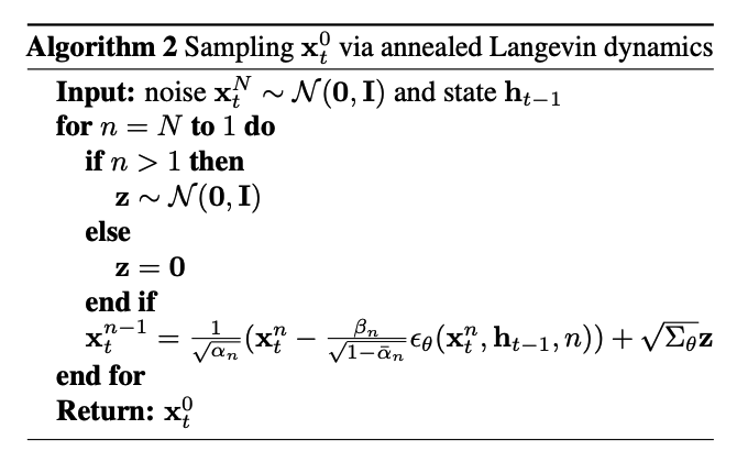
• obtain a sample \(\mathbf{x}_{T+1}^0\) of the next time step
• pass autoregressively to the RNN together with the covariates \(\mathbf{c}_{T+1}\)
  • obtain the next hidden state \(\mathbf{h}_{T+1}\)
  • repeat until the desired forecast horizon has been reached.

“warm-up” state \(\mathbf{h}_T\)

• can be repeated many times (e.g. \(S=100\) )
• to obtain empirical quantiles of the uncertainty of our predictions.

(3) Scaling

Magnitudes of different TS entities can vary drastically

\(\rightarrow\) Normalize it!

Divide each TS entity by their context window mean

( & Re-scale it at inference time )

4. Experiments

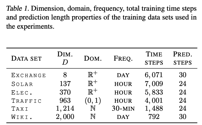
Datasets : 6 real-world datasets

(1) Evaluation Metric and Data Set

a) Metric

Continuous Ranked Probability Score (CRPS)

• \(\operatorname{CRPS}(F, x)=\int_{\mathbb{R}}(F(z)-\mathbb{I}\{x \leq z\})^2 \mathrm{~d} z,\).

Empirical CDF of \(F\)

• \(\hat{F}(z)=\frac{1}{S} \sum_{s=1}^S \mathbb{I}\left\{X_s \leq\right.\) \(z\}\) with \(S\) samples \(X_s \sim F\)

\(\operatorname{CRPS}_{\text {sum }}=\mathbb{E}_t\left[\operatorname{CRPS}\left(\hat{F}_{\text {sum }}(t), \sum_i x_{i, t}^0\right)\right]\).

= obtained by first summing across the \(D\) time-series

& averaged over the prediction horizon

b) Datasets