(paper 90) CSDI; Conditional Score-baesd Diffusion Models for Probabilistic TS Imputation

CSDI: Conditional Score-baesd Diffusion Models for Probabilistic TS Imputation

Contents

1. Abstract
2. Introduction
3. Related Works
   1. TS imputation with DL
   2. Score-based Generative models
4. Background
   1. MTS imputation
   2. Denoising diffusion probabilistic models
   3. Imputation with Diffusion models
5. CSDI
   1. Imputation with CSDI
   2. Training of CSDI
   3. Choice of imputation targets in SSL
6. Implementation of CSDI
7. Experimental Results
   1. TS Imputation

0. Abstract

AR models : natural for TS imputation

**Score-based diffusion models **: outperformed ARs, in…

• image generation and audio synthesis
• would be promising for TS imputation.

Conditional Score-based Diffusion models for Imputation (CSDI)

Novel TS imputation method

• utilizes score-based diffusion models conditioned on observed data
  • exploit correlations between observed values.
• explicitly trained for imputation

1. Introduction

Imputation methods based on DNN

• (1) Deterministic imputation
• (2) Probabilistic imputation

\(\rightarrow\) typically utilize AR models to deal with TS

Score-based diffusion models

can also be used to impute missing values

• by approximating the scores of the posterior distribution,

  obtained from the prior by conditioning on the observed values

• may work well in practice, they do not correspond to the exact conditional distribution.

CSDI

• a novel probabilistic imputation method
• directly learns the conditional distn with conditional score-based diffusion models
• designed for imputation & can exploit useful information in observed values.

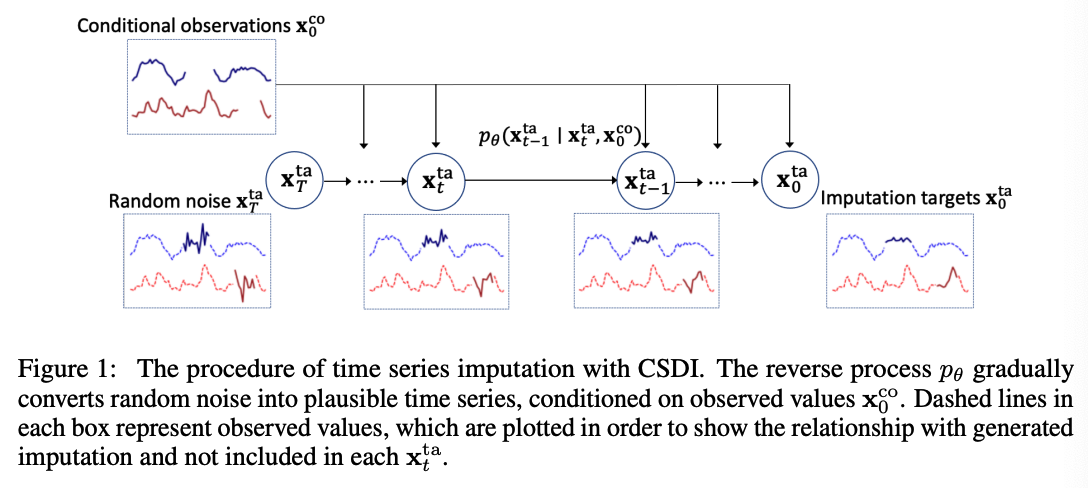
Overview

• Start imputation from random noise

• Gradually convert the noise into plausible TS

  • via reverse process \(p_\theta\) of the conditional diffusion model.

Reverse Process (at step \(t\))

• removes noise from the output of the previous step \((t+1)\).
• can take observations as a CONDITIONAL INPUT
  • exploit information in the OBSERVATIONS for denoising.
• utilize an attention mechanism
  • to capture the TERMPORAL & FEATURE dependencies of TS

Data

• observed values (i.e., conditional information)
• ground-truth missing values (i.e., imputation targets).

However, in practice we do not know the GT missing values

\(\rightarrow\) inspired by MLM, develop a SSL method

• that separates observed values into conditional information and imputation targets.

CSDI is formulated for general imputation tasks

( not restricted to TS imputation )

Contributions

1. Conditional score-based diffusion models for probabilistic imputation (CSDI)**
   • to train the conditional diffusion model, develop SSL method
2. Experiments
   • improves the continuous ranked probability score (CRPS)
   • decreases the mean absolute error (MAE)
3. Can be applied to TS interpolations and probabilistic forecasting

2. Related works

(1) TS imputation with DL

• RNN-based

• RNN + GANs/Self-training
• Combination of RNNs & attention mechanisms : successful

\(\rightarrow\) mostly focused on deterministic imputation

( \(\leftrightarrow\) GP-VAE : has been recently developed as a probabilistic imputation method )

(2) Score-based Generative models

Examples)

• score matching with Langevin dynamics

• denoising diffusion probabilistic models

outperformed existing methods with other deep generative models

TimeGrad

• utilized diffusion probabilistic models for probabilistic TS forecasting.
• BUT cannot be applied to TS imputation
  • due to the use of RNNs to handle past time series.

3. Background

(1) MTS imputation

Notation

• \(N\) MTS with missing values

  • each TS : \(\mathbf{X}=\left\{x_{1: K, 1: L}\right\} \in \mathbb{R}^{K \times L}\)

    • \(K\) : number of features

    • \(L\) : length of TS

      ( can be differnt for each TS ,but assume same )

• Observation mask : \(\mathbf{M}=\left\{m_{1: K, 1: L}\right\} \in\{0,1\}^{K \times L}\)
  • missing : \(m_{k, l}=0\)
  • observed : \(m_{k, l}=1\)
• Timestamps of TS as \(\mathbf{s}=\left\{s_{1: L}\right\} \in \mathbb{R}^L\)
  • Assume time intervals between two consecutive data entries can be different

\(\rightarrow\) Each TS is expressed as \(\{\mathbf{X}, \mathbf{M}, \mathbf{s}\}\).

Probabilistic TS imputation

= estimating the distn of the missing values of \(\mathbf{X}\)

• by exploiting the observed values of \(\mathbf{X}\).

Definition of imputation

• includes other related tasks
• ex) Interpolation
  • which imputes all features at TARGET time points
• ex) Forecasting
  • which imputes all features at FUTURE time points.

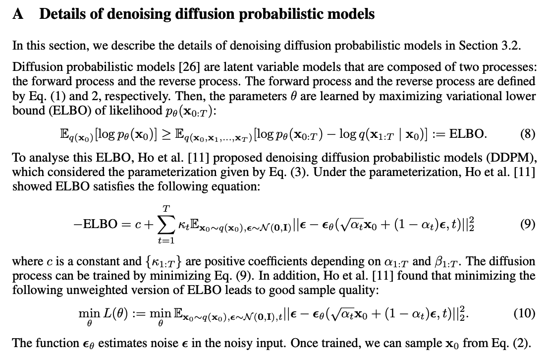
(2) Denoising diffusion probabilistic models

Learning a model distribution \(p_\theta\left(\mathbf{x}_0\right)\) that approximates a data distribution \(q\left(\mathbf{x}_0\right)\).

Diffusion probabilistic models

= latent variable models that are composed of two processes:

• (1) Forward process
• (2) Reverse process

a) Forward Process ( add noise )

( defined by Markov Chain )

\(q\left(\mathbf{x}_{1: T} \mid \mathbf{x}_0\right):=\prod_{t=1}^T q\left(\mathbf{x}_t \mid \mathbf{x}_{t-1}\right) \text { where } q\left(\mathbf{x}_t \mid \mathbf{x}_{t-1}\right):=\mathcal{N}\left(\sqrt{1-\beta_t} \mathbf{x}_{t-1}, \beta_t \mathbf{I}\right)\).

• \(\beta_t\) : small positive constant ( = noise level )

\(q\left(\mathbf{x}_t \mid \mathbf{x}_0\right)=\mathcal{N}\left(\mathbf{x}_t ; \sqrt{\alpha_t} \mathbf{x}_0,\left(1-\alpha_t\right) \mathbf{I}\right)\).

• where \(\hat{\alpha}_t:=1-\beta_t\) and \(\alpha_t:=\prod_{i=1}^t \hat{\alpha}_i\).

Thus, we can rewrite as …

\(\mathbf{x}_t=\sqrt{\alpha_t} \mathbf{x}_0+\left(1-\alpha_t\right) \boldsymbol{\epsilon}\) where \(\boldsymbol{\epsilon} \sim \mathcal{N}(\mathbf{0}, \mathbf{I})\).

b) Reverse Process ( denoise )

( defined by Markov Chain )

Denoises \(\mathbf{x}_t\) to recover \(\mathbf{x}_0\)

\(\begin{aligned} & p_\theta\left(\mathbf{x}_{0: T}\right):=p\left(\mathbf{x}_T\right) \prod_{t=1}^T p_\theta\left(\mathbf{x}_{t-1} \mid \mathbf{x}_t\right), \quad \mathbf{x}_T \sim \mathcal{N}(\mathbf{0}, \mathbf{I}), \\ & p_\theta\left(\mathbf{x}_{t-1} \mid \mathbf{x}_t\right):=\mathcal{N}\left(\mathbf{x}_{t-1} ; \boldsymbol{\mu}_\theta\left(\mathbf{x}_t, t\right), \sigma_\theta\left(\mathbf{x}_t, t\right) \mathbf{I}\right) \end{aligned}\).

Denoising diffusion probabilistic models (DDPM)

Specific parameterization of \(p_\theta\left(\mathbf{x}_{t-1} \mid \mathbf{x}_t\right)\) :

\(\boldsymbol{\mu}_\theta\left(\mathbf{x}_t, t\right)=\frac{1}{\alpha_t}\left(\mathbf{x}_t-\frac{\beta_t}{\sqrt{1-\alpha_t}} \boldsymbol{\epsilon}_\theta\left(\mathbf{x}_t, t\right)\right), \sigma_\theta\left(\mathbf{x}_t, t\right)=\tilde{\beta}_t^{1 / 2} \text { where } \tilde{\beta}_t= \begin{cases}\frac{1-\alpha_{t-1}}{1-\alpha_t} \beta_t & t>1 \\ \beta_1 & t=1\end{cases}\).

• where \(\boldsymbol{\epsilon}_\theta\) is a trainable denoising function.

Denote as..

• \(\boldsymbol{\mu}_\theta\left(\mathbf{x}_t, t\right)\) \(\rightarrow\) \(\boldsymbol{\mu}^{\mathrm{DDPM}}\left(\mathbf{x}_t, t, \boldsymbol{\epsilon}_\theta\left(\mathbf{x}_t, t\right)\right)\)
• \(\sigma_\theta\left(\mathbf{x}_t, t\right)\) \(\rightarrow\) \(\sigma^{\mathrm{DDPM}}\left(\mathbf{x}_t, t\right)\)

Corresponds to a rescaled score model for score-based generative models

Ho et al. [11] have shown that ….

the reverse process can be trained by solving the following optimization problem:

\(\min _\theta \mathcal{L}(\theta):=\min _\theta \mathbb{E}_{\mathbf{x}_0 \sim q\left(\mathbf{x}_0\right), \boldsymbol{\epsilon} \sim \mathcal{N}(\mathbf{0}, \mathbf{I}), t}\left\|\boldsymbol{\epsilon}-\boldsymbol{\epsilon}_\theta\left(\mathbf{x}_t, t\right)\right\|_2^2 \quad \text { where } \mathbf{x}_t=\sqrt{\alpha_t} \mathbf{x}_0+\left(1-\alpha_t\right) \boldsymbol{\epsilon}\).

Summary of above :

• denoising function \(\epsilon_\theta\) estimates the noise vector \(\epsilon\) that was added to its noisy input \(\mathbf{x}_t\).
• can also be viewed as a weighted combination of denoising score matching used for training score-based generative models

(3) Imputation with Diffusion models

Focus on general imputation tasks

( not restricted to TS imputation )

Imputation problem

• given a sample \(\mathbf{x}_0\) with missing values, generate imputation targets \(\mathbf{x}_0^{\mathrm{ta}} \in \mathcal{X}^{\text {ta }}\)

  • by exploiting conditional observations \(\mathbf{x}_0^{\text {co }} \in \mathcal{X}^{\text {co }}\),

• Goal of probabilistic imputation

  = estimate the true conditional data distn \(q\left(\mathbf{x}_0^{\mathrm{ta}} \mid \mathbf{x}_0^{\text {co }}\right)\) with a model distn \(p_\theta\left(\mathbf{x}_0^{\text {ta }} \mid \mathbf{x}_0^{\text {co }}\right)\).

• typically impute all missing values using all observed values

  • set all observed values as \(\mathbf{x}_0^{\text {co }}\)
  • set all missing values as \(\mathbf{x}_0^{\text {ta }}\)

Modeling \(p_\theta\left(\mathbf{x}_0^{\text {ta }} \mid \mathbf{x}_0^{\text {co }}\right)\) with a diffusion model

• case 1) Unconditional )

  • Reverse process \(p_\theta\left(\mathbf{x}_{0: T}\right)\) is used to define the final data model \(p_\theta\left(\mathbf{x}_0\right)\).

• case 2) Conditional )

  • extend the reverse process in case 1)

    \(\begin{aligned} & p_\theta\left(\mathbf{x}_{0: T}^{\mathrm{ta}} \mid \mathbf{x}_0^{\mathrm{co}}\right):=p\left(\mathbf{x}_T^{\mathrm{ta}}\right) \prod_{t=1}^T p_\theta\left(\mathbf{x}_{t-1}^{\mathrm{ta}} \mid \mathbf{x}_t^{\mathrm{ta}}, \mathbf{x}_0^{\mathrm{co}}\right), \quad \mathbf{x}_T^{\mathrm{ta}} \sim \mathcal{N}(\mathbf{0}, \mathbf{I}), \\ & p_\theta\left(\mathbf{x}_{t-1}^{\mathrm{ta}} \mid \mathbf{x}_t^{\mathrm{ta}}, \mathbf{x}_0^{\mathrm{co}}\right):=\mathcal{N}\left(\mathbf{x}_{t-1}^{\mathrm{ta}} ; \boldsymbol{\mu}_\theta\left(\mathbf{x}_t^{\mathrm{ta}}, t \mid \mathbf{x}_0^{\mathrm{co}}\right), \sigma_\theta\left(\mathbf{x}_t^{\mathrm{ta}}, t \mid \mathbf{x}_0^{\mathrm{co}}\right) \mathbf{I}\right) \end{aligned}\).

Existing diffusion models

• generally designed for data generation
• do not take conditional observations \(\mathbf{x}_0^{\text {co }}\) as inputs.

4. Conditional score-based diffusion model for imputation (CSDI)

Novel imputation method based on a conditional score-based diffusion model

• Allows us to exploit useful information in observed values for accurate imputation.

• Provide the reverse process of the conditional diffusion model

• Develop a SSL training method.

• Not restricted to TS

(1) Imputation with CSDI

Model the conditional distribution \(p\left(\mathbf{x}_{t-1}^{\mathrm{ta}} \mid \mathbf{x}_t^{\mathrm{ta}}, \mathbf{x}_0^{\text {co }}\right)\) without approximations.

• Extend the parameterization of DDPM to the conditional case.

Conditional denoising function \(\boldsymbol{\epsilon}_\theta:\left(\mathcal{X}^{\mathrm{ta}} \times \mathbb{R} \mid \mathcal{X}^{\mathrm{co}}\right) \rightarrow \mathcal{X}^{\mathrm{ta}}\)

• takes conditional observations \(\mathbf{x}_0^{\text {co }}\) as inputs.

Parameterization with \(\epsilon_\theta\) :

• \(\boldsymbol{\mu}_\theta\left(\mathbf{x}_t^{\mathrm{ta}}, t \mid \mathbf{x}_0^{\mathrm{co}}\right)=\boldsymbol{\mu}^{\mathrm{DDPM}}\left(\mathbf{x}_t^{\mathrm{ta}}, t, \boldsymbol{\epsilon}_\theta\left(\mathbf{x}_t^{\mathrm{ta}}, t \mid \mathbf{x}_0^{\mathrm{co}}\right)\right)\).
• \(\sigma_\theta\left(\mathbf{x}_t^{\mathrm{ta}}, t \mid \mathbf{x}_0^{\mathrm{co}}\right)=\sigma^{\mathrm{DDPM}}\left(\mathbf{x}_t^{\mathrm{ta}}, t\right)\).

( where \(\boldsymbol{\mu}^{\mathrm{DDPM}}\) and \(\sigma^{\mathrm{DDPM}}\) are the functions defined in Section 3.2 )

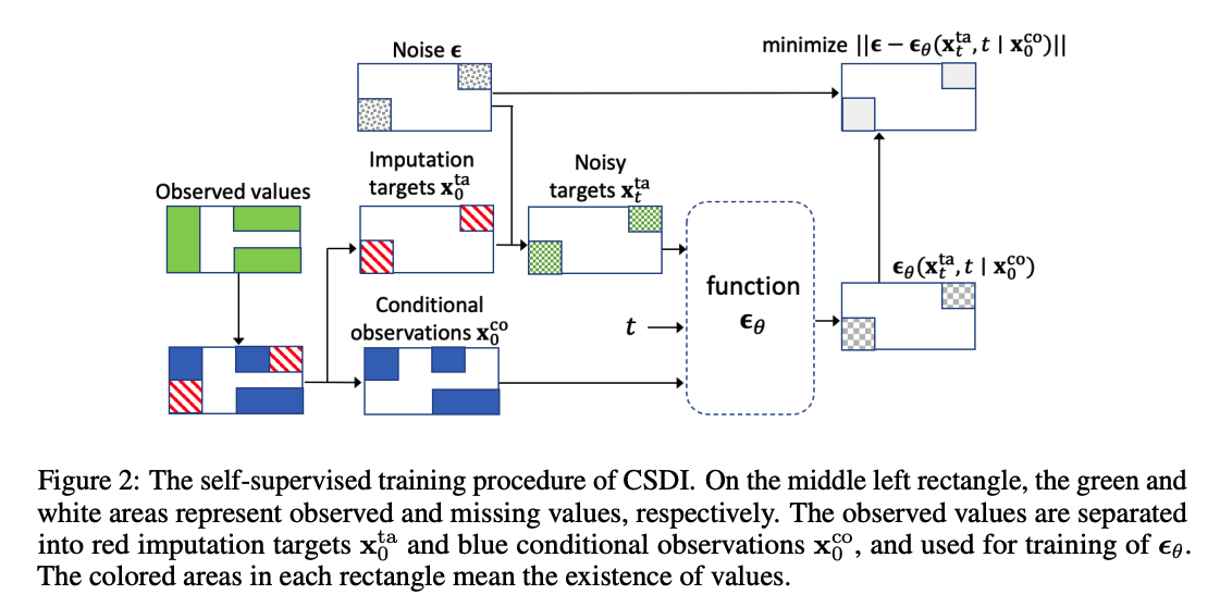
(2) Training of CSDI

Given ….

• (1) conditional observations \(\mathbf{x}_0^{\text {co }}\)
• (2) imputation targets \(\mathbf{x}_0^{\mathrm{ta}}\)

Sample noisy targets \(\mathbf{x}_t^{\mathrm{ta}}=\sqrt{\alpha_t} \mathbf{x}_0^{\mathrm{ta}}+\left(1-\alpha_t\right) \boldsymbol{\epsilon}\)

Train \(\boldsymbol{\epsilon}_\theta\) by minimizing …

• \(\min _\theta \mathcal{L}(\theta):=\min _\theta \mathbb{E}_{\mathbf{x}_0 \sim q\left(\mathbf{x}_0\right), \boldsymbol{\epsilon} \sim \mathcal{N}(\mathbf{0}, \mathbf{I}), t}\left\|\left(\boldsymbol{\epsilon}-\boldsymbol{\epsilon}_\theta\left(\mathbf{x}_t^{\mathrm{ta}}, t \mid \mathbf{x}_0^{\mathrm{co}}\right)\right)\right\|_2^2\).
  • dim of \(\epsilon\) corresponds to that of the imputation targets \(\mathbf{x}_0^{\mathrm{ta}}\).

Problem?

do not know the ground-truth missing values in practice!!

• not clear how to select \(\mathbf{x}_0^{\text {co }}\) and \(\mathbf{x}_0^{\text {ta }}\) from a training sample \(\mathbf{x}_0\).

\(\rightarrow\) Develop a SSL method ( inspired by MLM )

(3) Choice of imputation targets in SSL

Choice of imputation targets is important!

Provide FOUR target choice strategies

• depending on what is known about the missing patterns in the test dataset.

(1) Random strategy :

• used when we do not know about missing patterns
• The percentage is sampled from \([0 \%, 100 \%]\)
  • to adapt to various missing ratios in the test dataset.

(2) Historical strategy :

• exploits missing patterns in the training dataset.

• Procedure

  • Given a training sample \(\mathbf{x}_0\), we randomly draw another sample \(\tilde{\mathbf{x}}_0\) from the training dataset.

  • Set the intersection of

    • the observed indices of \(\mathbf{x}_0\)
    • the missing indices of \(\tilde{\mathbf{x}}_0\)

    as imputation targets.

(3) Mix strategy :

• mix of the above two strategies.
  • historical strategy : may lead to overfitting

(4) Test pattern strategy :

• when we know the missing patterns in the test dataset
• ex) used for TS forecasting
  • since the missing patterns in the test dataset are fixed to given future time points.

5. Implementation of CSDI for time series imputation

Sample space \(\mathcal{X}\) of \(\mathbf{X}\) : \(\mathbb{R}^{K \times L}\).

Want to handle \(\mathbf{X}\) in the sample space \(\mathbb{R}^{K \times L}\)

\(\rightarrow\) But the conditional denoising function \(\epsilon_\theta\) takes inputs \(\mathbf{x}_t^{\mathrm{ta}}\) and \(\mathbf{x}_0^{\mathrm{co}}\) in varying sample spaces

\(\rightarrow\) To address this issue, adjust inputs in the fixed sample space \(\mathbb{R}^{K \times L}\)

How to fix?

• Fix the shape of the inputs \(\mathbf{x}_t^{\text {ta }}\) and \(\mathbf{x}_0^{\text {co }}\) to \((K \times L)\) by applying zero padding to \(\mathbf{x}_t^{\text {ta }}\) and \(\mathbf{x}_0^{\text {co }}\).

  ( = set zero values to white areas for \(\mathbf{x}_t^{\text {ta }}\) and \(\mathbf{x}_0^{\text {co }}\) )

  ( + introduce the conditional mask \(\mathbf{m}^{\mathrm{co}} \in\{0,1\}^{K \times L}\) )

• For ease of handling, we also fix the output shape in the sample space \(\mathbb{R}^{K \times L}\) by applying zero padding

Result : Conditional denoising function : \(\boldsymbol{\epsilon}_\theta\left(\mathbf{x}_t^{\mathrm{ta}}, t \mid \mathbf{x}_0^{\mathrm{co}}, \mathbf{m}^{\text {co }}\right)\)

• can be written as \(\boldsymbol{\epsilon}_\theta:\left(\mathbb{R}^{K \times L} \times \mathbb{R} \mid \mathbb{R}^{K \times L} \times\{0,1\}^{K \times L}\right) \rightarrow \mathbb{R}^{K \times L}\).

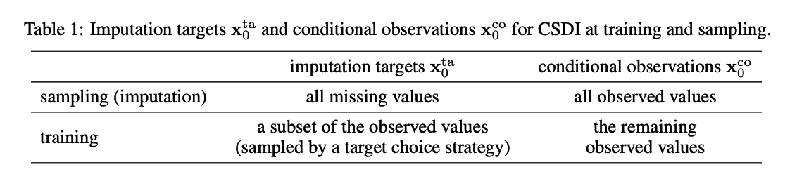
[ Sampling ( = Inference ) ]

• since conditional observations \(\mathbf{x}_0^{\text {co }}\) are all observed values …
• set \(\mathbf{m}^{\text {co }}=\mathbf{M}\) and \(\mathbf{x}_0^{\text {co }}=\mathbf{m}^{\text {co }} \odot \mathbf{X}\)

[ Training ]

• sample \(\mathbf{x}_0^{\text {ta }}\) and \(\mathbf{x}_0^{\text {co }}\) through a target choice strategy
• Then, \(\mathbf{x}_0^{\text {co }}\) is written as \(\mathbf{x}_0^{\text {co }}=\mathbf{m}^{\text {co }} \odot \mathbf{X}\) and \(\mathbf{x}_0^{\mathrm{ta}}\) is obtained as \(\mathbf{x}_0^{\mathrm{ta}}=\left(\mathbf{M}-\mathbf{m}^{\mathrm{co}}\right) \odot \mathbf{X}\).

Architecture of \(\epsilon_\theta\).

• adopt the architecture in DiffWave
  • composed of multiple residual layers with residual channel \(C\).
• refine this architecture for TS imputation.
  • set the diffusion step \(T=50\).

Attention mechanism

to capture temporal and feature dependencies of MTS

\(\rightarrow\) utilize 2-dim attention mechanism ( in each residual layer ) instead of CNN

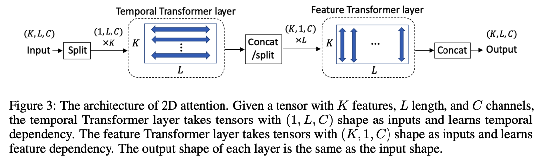
Architecture ( both 1-layer Transformer encoders )

• Temporal Transformer layer
  • takes tensors for each feature as inputs to learn temporal dependency
• Feature Transformer layer
  • takes tensors for each time point as inputs to learn temporal dependency.

While the length \(L\) can be different for each TS, attention mechanism allows the model to handle various lengths. ( For batch training,apply zero padding to each sequence )

Side Information

provide side information as additional input

• (1) Time embedding of \(\mathbf{s}=\left\{s_{1: L}\right\}\) ( dim = 128 )
• (2) Categorical feature embedding for \(K\) features ( dim = 16 )

6. Experimental results

Can be applied to other related tasks

• ex) interpolation and forecasting

\(\rightarrow\) Evaluate CSDI for these tasks to show the flexibility of CSDI.

(1) Time series imputation

2 datasets

a) PhysioNet Challenge 2012

• healthcare dataset

  ( 4000 clinical time series with 35 variables for 48 hours from intensive care unit (ICU) )

• process the dataset to hourly time series with 48 time steps.

• \(80 \%\) missing values. ( no GT )

• But no GT ..

  \(\rightarrow\) Evaluation : randomly choose \(10 / 50 / 90 \%\) of observed values as GT on the test data.

b) Air quality

• use hourly sampled PM2.5 measurements from 36 stations in Beijing for 12 months and set 36 consecutive time steps as one time series.
• \(13 \%\) missing values ( + missing patterns are not random )
• Artificial GT
  • whose missing patterns are also structured.

Details:

• Run for 5 times

• Target choice strategy :

  • a) PhysioNet : random strategy

  • b) Air quality : mix of the random and historical strategy

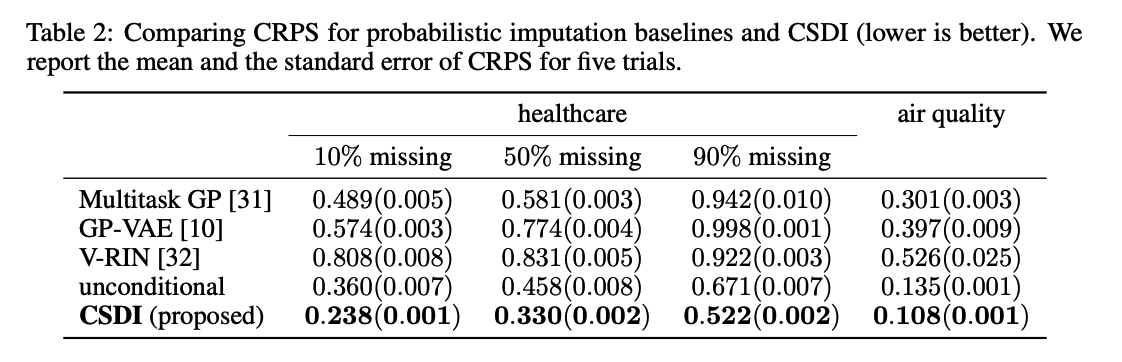
Results of probabilistic imputation

Four baselines.

• (1) Multitask GP: learns the covariance between timepoints & features simultaneously.
• (2) GP-VAE : SOTA for probabilistic imputation.
• (3) V-RIN : a deterministic imputation method
  • uses the uncertainty quantified by VAE to improve imputation.
  • regard the quantified uncertainty as probabilistic imputation.
• (4) Unconditional diffusion model

Metric : continuous ranked probability score (CRPS)

• used for evaluating probabilistic time series forecasting
• measures the compatibility of an estimated probability distribution with an observation

Generate 100 samples to approximate the probability distribution over missing values

& Report the normalized average of CRPS for all missing values