[ 6. Graph Neural Networks ]Permalink

( 참고 : CS224W: Machine Learning with Graphs )

ContentsPermalink

• 6-1. Introduction
• 6-2. DL for graphs
• 6-3. GCN (Graph Convolution Networks)
• 6-4. GNN vs CNN
• 6-5. GNN vs Transformer

6-1. IntroductionPermalink

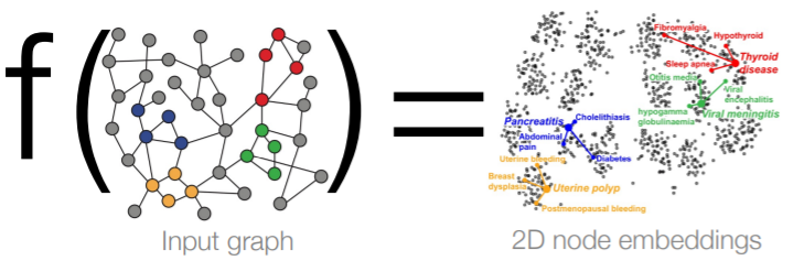
learn mapping function via NN!

• similar nodes, close in embedding space

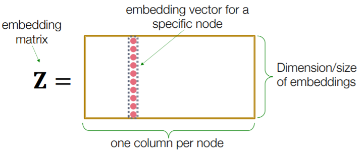
Shallow Encoders

• just “embedding-lookup table”
• limitations :
  • 1) $O(\mid V \mid)$ parameters needed
  • 2) “transductive”
    • no embeddings for unseen nodes
  • 3) do not use “node features”

Networks are complex!

• arbitrary size & complex topological structure
• no fixed node ordering / reference point
• dynamic & multimodal features

6-2. DL for graphsPermalink

Notation

• $V$ : vertex set
• $A$ : adjacency matrix
• $\boldsymbol{X} \in \mathbb{R}^{m \times \mid V \mid}$ : matrix of “node features”
• $N(v)$ : neighbors of node $v$

Naive approach : use concat ( [$A$ , $X$] ) as input

CNN : problems?

• no fixed notion of locality or sliding window on the graph

  ( there can be many order plans :( )

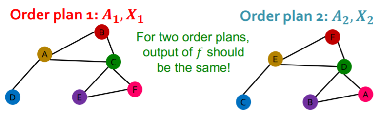
(1) Permutation invariant functionPermalink

• input graph : $G=(\boldsymbol{A}, \boldsymbol{X})$

• map $G$ into vector $\mathbb{R}^{d}$

• $f$ is “Permutation invariant function”,

  if $f\left(\boldsymbol{A}_{i}, \boldsymbol{X}_{i}\right)=f\left(\boldsymbol{A}_{j}, \boldsymbol{X}_{j}\right)$ for any order plan $i$ &$j$

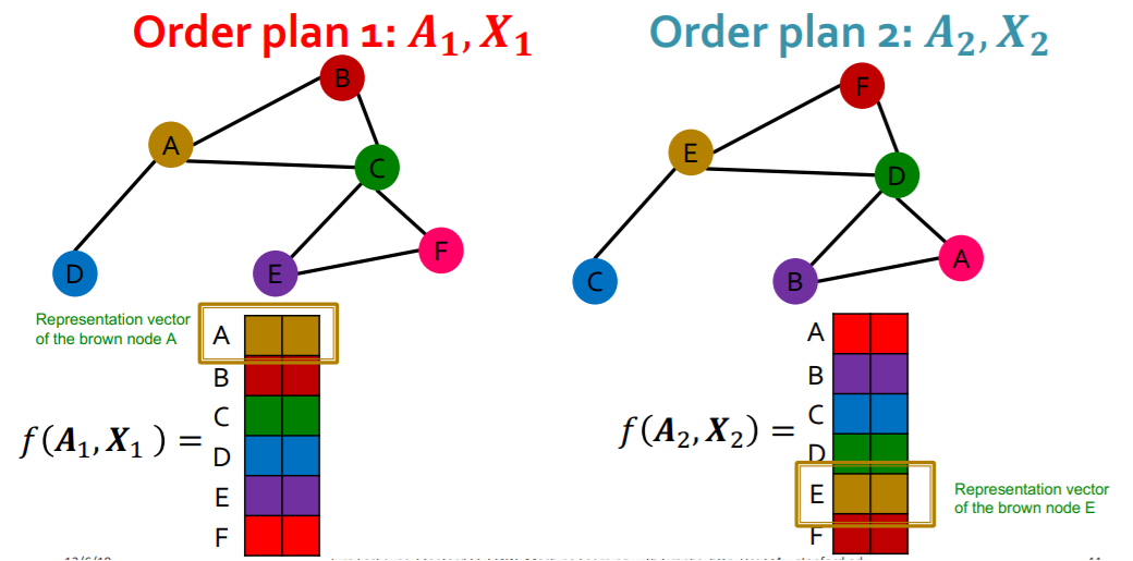
(2) Permutation EquivariancePermalink

for 2 order plans..

the vector of “SAME POSITION” should have “SAME EMBEDDING”

(3) GNNPermalink

GNN consists of multiple…

• 1) permutation “invariant” layers
• 2) permutation “equivariant” layers

( but naive MLP’s do not meet those conditions! )

So, how to design “invariant & equivariant” layers?

6-3. GCN (Graph Convolution Networks)Permalink

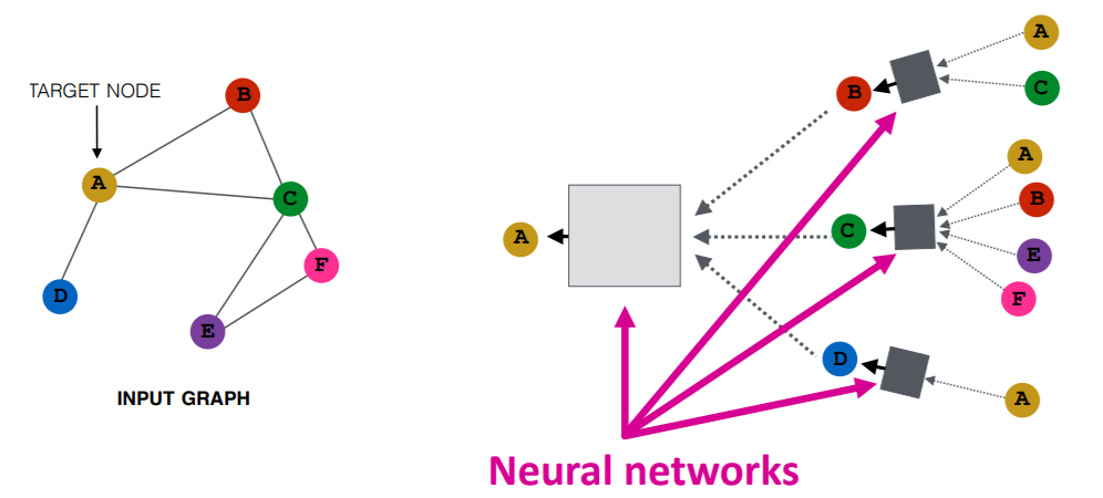
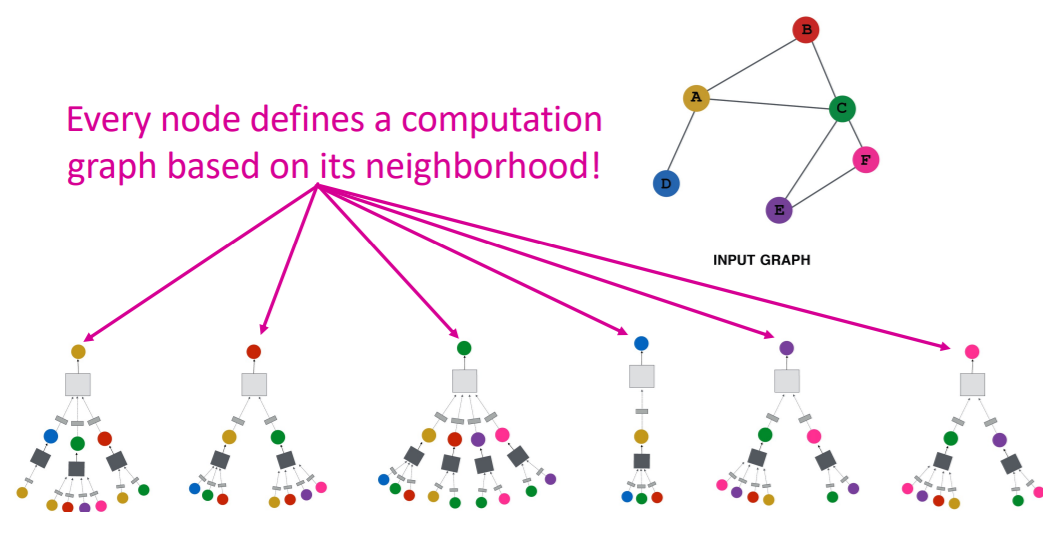
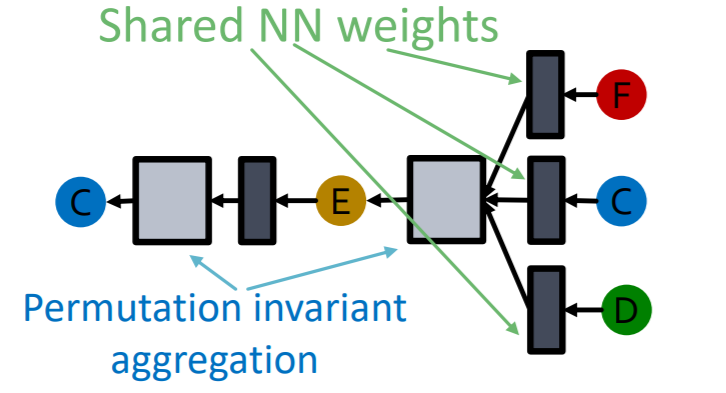
(1) Basic IdeaPermalink

• Node’s neighborhood defines a computation graph
• so, how to propagate neighbor’s information?

Let’s generate node embeddings,

• based on “LOCAL NETWORK NEIGHBORHOOD”
• by using NN

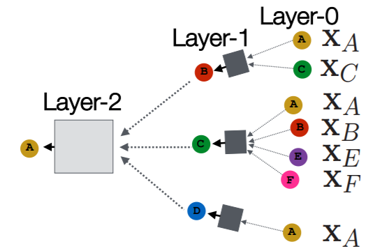
(2) Depth of NNPermalink

meaning of “Depth” ( of layers )

• layer 0 : target node itself
• layer 1 : 1-hop neighbors
• …
• layer $K$ : $K$-hops neighbors

(3) Neighborhood aggregationPermalink

Procedure

• step 1) average messages of neighbors

• step 2) apply NN

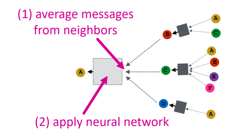
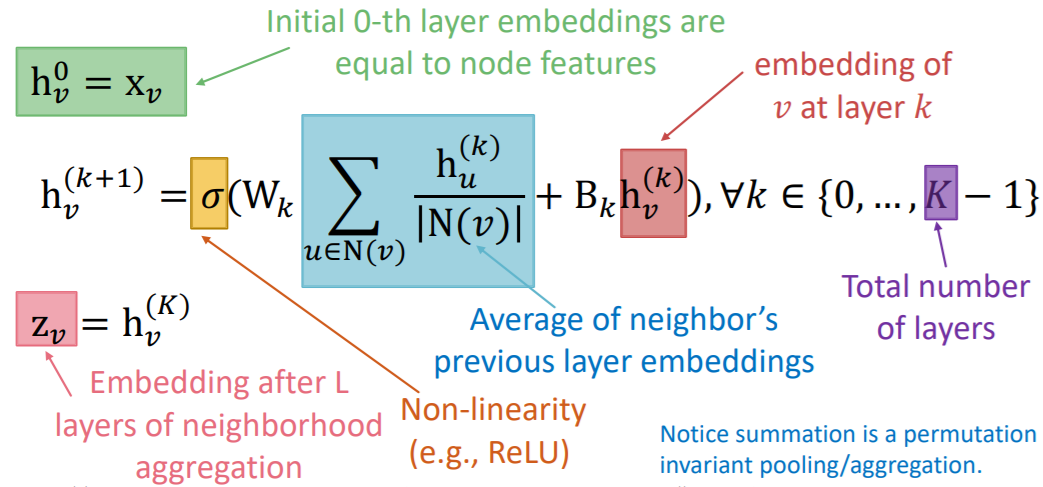
Both steps are “permutation equivariant”

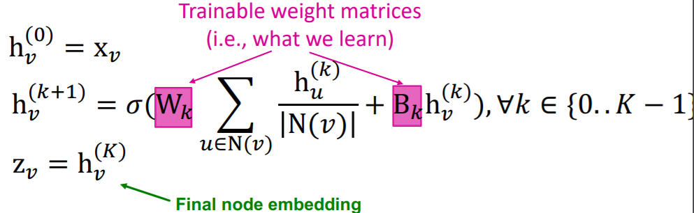
(4) Training GCNPermalink

2 big steps

• 1) defining “neighborhood aggregation” function
• 2) defining “loss function”

Notation

• $h_v^k$ : hidden representation of $v$ at layer $k$
  • $W_k$ : parameter for “neighborhood aggregation”
  • $B_k$ : parameter for “transforming itself”

(5) Matrix FormulationPermalink

We can solve the above, by “matrix formulation”

• (vector) $\sum_{u \in N(v)} \frac{h_{u}^{(k-1)}}{\mid N(v) \mid}$.

• (matrix) $H^{(k+1)}=D^{-1} A H^{(k)}$.

  • $H^{(k)}=\left[h_{1}^{(k)} \ldots h_{ \mid V \mid }^{(k)}\right]^{\mathrm{T}}$.

    ( thus, $\sum_{u \in N_{v}} h_{u}^{(k)}=\mathrm{A}_{v,:} \mathrm{H}^{(k)}$ )

  • $D_{v, v}=\operatorname{Deg}(v)= \mid N(v) \mid$.

Updating FunctionPermalink

$H^{(k+1)}=\sigma\left(\tilde{A} H^{(k)} W_{k}^{\mathrm{T}}+H^{(k)} B_{k}^{\mathrm{T}}\right)$.

• where $\tilde{A}=D^{-1} A$
• term 1) $\tilde{A} H^{(k)} W_{k}^{\mathrm{T}}$ :neighborhood aggregation
• term 2) $H^{(k)} B_{k}^{\mathrm{T}}$ : self-transformation

Unsupervised TrainingPermalink

Loss Function :

$\mathcal{L}=\sum_{z_{u}, z_{v}} \operatorname{CE}\left(y_{u, v}, \operatorname{DEC}\left(z_{u}, z_{v}\right)\right)$.

• $y_{u,v}=1$, if $u$ and $v$ is similar
• example of $DEC$ : inner product

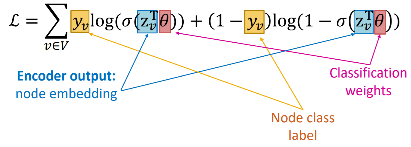
Supervised TrainingPermalink

just train as simple classification task!

( with CE loss )

General Training procedurePermalink

dataset : batch of sub-graphs

procedure

• 1) train on a set of nodes
• 2) generate embedding “for all nodes”

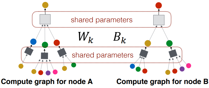
Note

• “same” aggregation parameters for “all nodes”

  $\rightarrow$ can generalize to UNSEEN nodes

6-4. GNN vs CNNPermalink

GNN :

• $\mathrm{h}_{v}^{(l+1)}=\sigma\left(\mathbf{W}_{l} \sum_{u \in \mathrm{N}(v)} \frac{\mathrm{h}_{u}^{(l)}}{ \mid \mathrm{N}(v) \mid }+\mathrm{B}_{l} \mathrm{~h}_{v}^{(l)}\right), \forall l \in\{0, \ldots, L-1\}$.

CNN :

• $\mathrm{h}_{v}^{(l+1)}=\sigma\left(\sum_{u \in \mathrm{N}(v)} \mathbf{W}_{l}^{u} \mathrm{~h}_{u}^{(l)}+\mathrm{B}_{l} \mathrm{~h}_{v}^{(l)}\right), \forall l \in\{0, \ldots, L-1\}$.

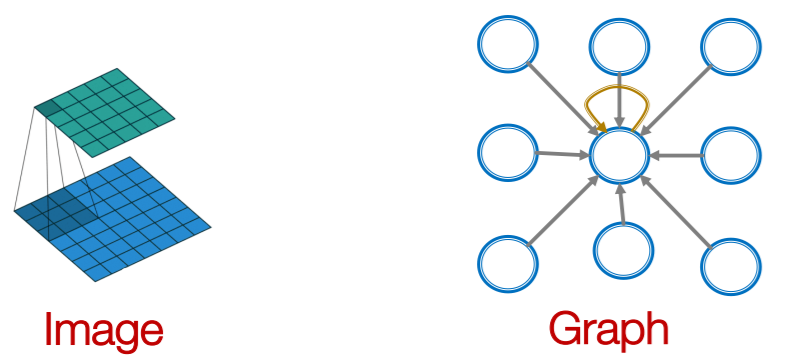
Intuition

• learn “DIFFERENT” $W_l$ for “DIFFERENT” neighbors in CNN,

  but not in GNN

  ( $\because$ can pick an “ORDER” of neighbors, using “RELATIVE position”)

• can think of CNN as an “special GNN, with fixed neighbor size & ordering”

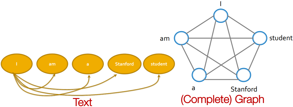
6-5. GNN vs TransformerPermalink

Transformer :

• can be seen as a special GNN that “runs on a fully connected word graph”