(CS224W) 5.Label Propagation for Node Classification

[ 5. Label Propagation for Node Classification ]

( 참고 : CS224W: Machine Learning with Graphs )

Contents

• 5-1. Message Passing and Node Classification
• 5-2. Node Correlation in networks
• 5-3. Relational Classification
• 5-4. Iterative Classification
• 5-5. Collective Classification ( Correct & Smooth )

5-1. Message Passing and Node Classification

Semi-supervised node classification

• some are LABELED
• some are UNLABELED
  • predict (=assign) labels with the LABELED ones

framework : Message passing

• intuition ) CORRELATION exists in the network
• Collective classification
  • assign labels to nodes “together”
• 3 techniques
  • 1) Relational Classification
  • 2) Iterative Classification
  • 3) Collective Classification ( correct & smooth )

5-2. Node Correlation in networks

why are nodes correlated?

• 1) homophily : individual —-(affect)—-> social
  • play with friends who are similar to me
  • ex) online social network
    • node : people
    • edge : friendship
    • node color : interests
• **2) influence **: social—-(affect)—-> individual
  • group’s atmosphere affect the individual inside the group

label of node \(v\) may depend on…

• 1) features of \(v\)
• 2) label of \(N(v)\)
• 3) features of \(N(v)\)

Semi-supervised task

• 1) settings : graph & (few) labeled nodes
• 2) goal : assign labels to UNlabeled nodes
• 3) assumption : homophily in the network

Notation

• \(A\) : \(n \times n\) adjacency matrix
• \(Y =\{0,1\}^n\) : vector of labels
  • \(Y_v =1\) , if node \(v\) belongs to class 1
  • \(Y_v =0\) , if node \(v\) belongs to class 0
• \(f_v\) : feature of node \(v\)
• task : find \(P(Y_v)\) , given all features in the network!

Will focus on “Semi-supervised Binary node classification”

• 1) Relational Classification
• 2) Iterative Classification
• 3) Collective Classification ( correct & smooth )

5-3. Relational Classification

(1) Probabilistic Relational Classifier

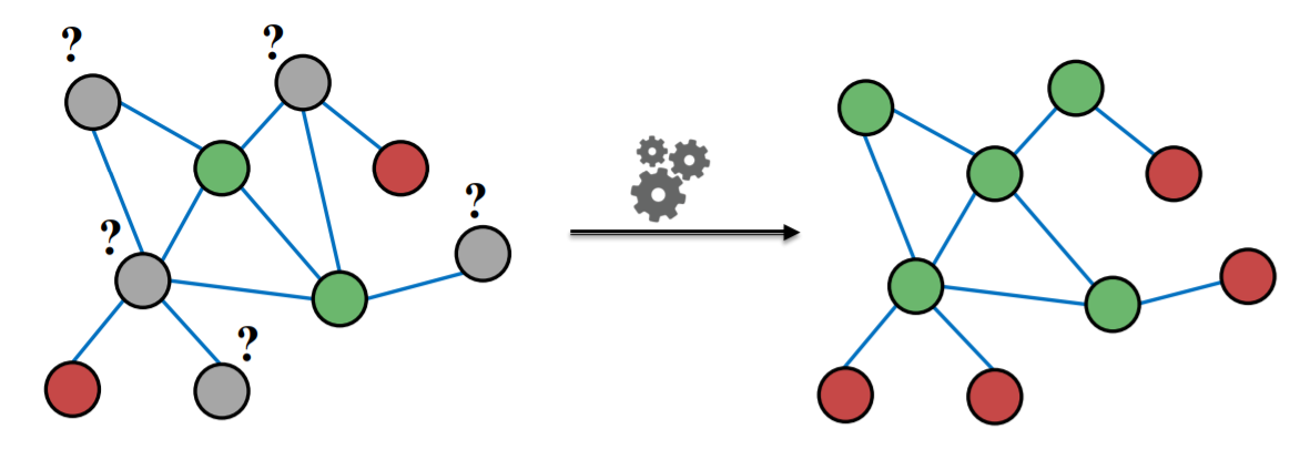
Idea : ‘propagate’ node labels

• \(Y_v\) : weighted average of \(Y_n\)s, where \(n\) are the neighbors

Initialization

• labeled nodes : ground truth label \(Y_v^{*}\)
• unlabeled nodes : \(Y_v=0.5\)

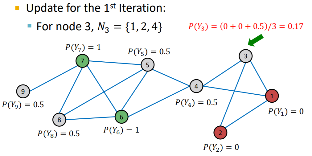
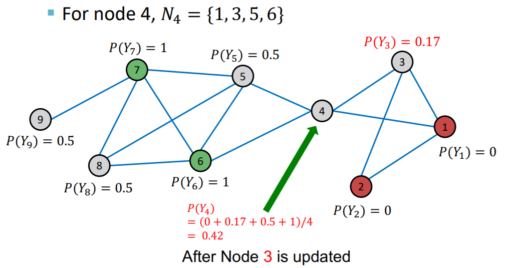
Update

• for each node \(v\) & label \(c\) ( 0 or 1 ) …

  \(P\left(Y_{v}=c\right)=\frac{1}{\sum_{(v, u) \in E} A_{v, u}} \sum_{(v, u) \in E} A_{v, u} P\left(Y_{u}=c\right)\).

  • \(P\left(Y_{v}=c\right)\) : prob of node \(v\) having label \(c\)
  • \(A_{v,u}\) : weight of edge between node \(v\) & \(u\)

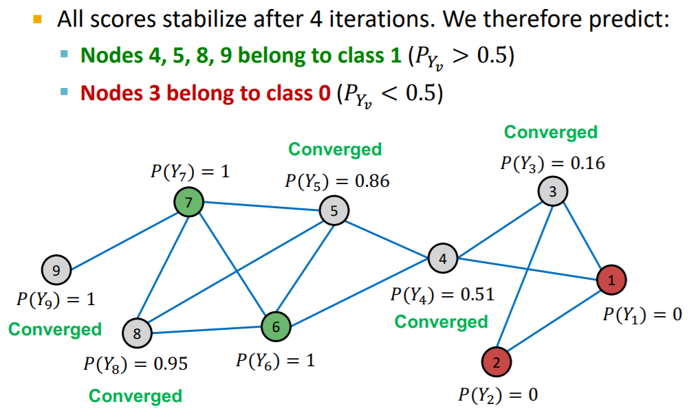
• problem :

  • convergence is not guaranteed
  • do not use node features

Process

…

5-4. Iterative Classification

(1) Key point

• use “node attribute \(f\) “
• classify label of node \(v\), based on..
  • 1) \(f_v\) ( = node attribute of \(v\) )
  • 2) \(z_v\) ( = labels of neighbor set \(N_v\) )

(2) Approach : train 2 classifiers!

• 1) \(\phi_1(f_v)\) : base classifier
• 2) \(\phi_2(f_v,z_v)\) : relational classifier
  • summary \(z_v\) of labels of \(N_v\)

(3) Summary \(z_v\)

example )

• 1) histogram of # of each label in \(N_v\)
• 2) most common label in \(N_v\)
• 3) # of different labels in \(N_v\)

(4) Architecture

Phase 1 : Classify, based on “NODE ATTRIBUTE” alone

• with “LABELED” dataset, train 2 models
  • 1) base classifier
  • 2) relational classifier

Phase 2 : Iterate, until convergence

• with “TEST” dataset,
  • 1) set \(Y_v\) based on “base classifier”
  • 2) compute \(z_v\) & predict \(\hat{Y_v}\) with “relational classifier”
• for (i in ALL_NODES):
  • step 1) update \(z_v\) with \(Y_u\) ( where \(u \in N_v\) )
  • step 2) update \(Y_v\), with \(z_v\)
  • ( iterate until max number / convergence )

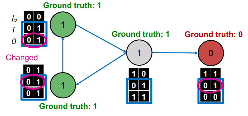
(5) Example : Web Page classification

Input : graph of web page

• node : web page
  • node features : web page description
• edge : hyper-link

Output : topic of the web-page

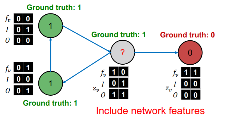
What will we use as \(z_v\) ( summary ) ?

• \(I\) : INCOMING neighbor label
• \(O\) : OUTGOING neighbor label

Procedure

step 1)

• train 2 classifiers ( with LABELED nodes )

• with trained \(\phi_1\), set \(Y_v\) for UNLABELED nodes

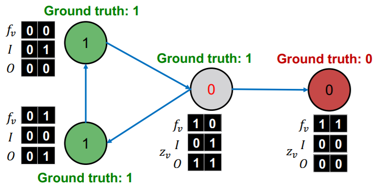
step 2)

• update \(z_v\) ( for ALL nodes )

step 3)

• re-classify with \(\phi_2\) ( for ALL nodes )

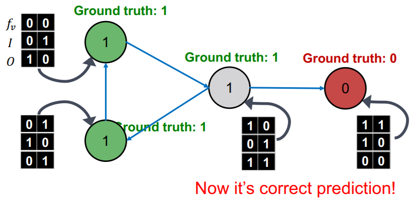
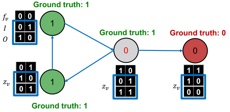
continue, until convergence

• 1) update \(z_v\) ( based on \(Y_v\) )
• 2) update \(Y_v\) ( = \(\phi_2(f_v,z_v)\) )

5-5. Collective Classification

C&S ( Correct & Smooth )

• SOTA collective classification

settings : “partially” labeled graph & features

Procedures

• step 1) train “BASE” predictor
• step 2) predict “SOFT LABELS” of ALL nodes with “BASE” predictor
• step 3) “POST-process” the prediction to get final result

(step 1) train base predictor

• predict “soft” labels with classifier ( ex. MLP )

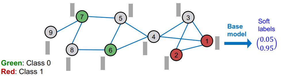
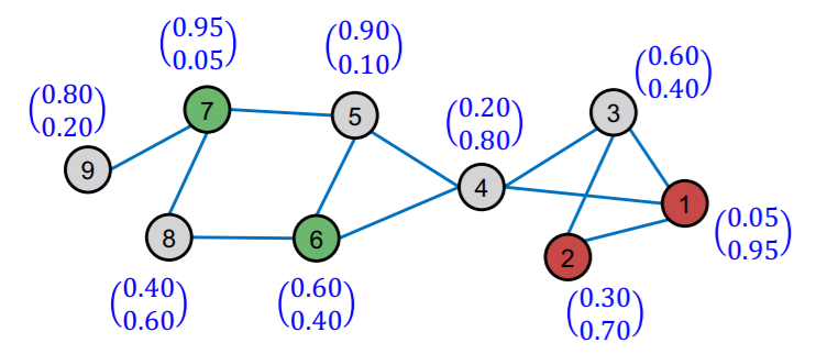
(step 2) predict all nodes

• obtain “soft” labels for all nodes

(step 3) post-process predictions

2 steps

• 1) correct step
• 2) smooth step

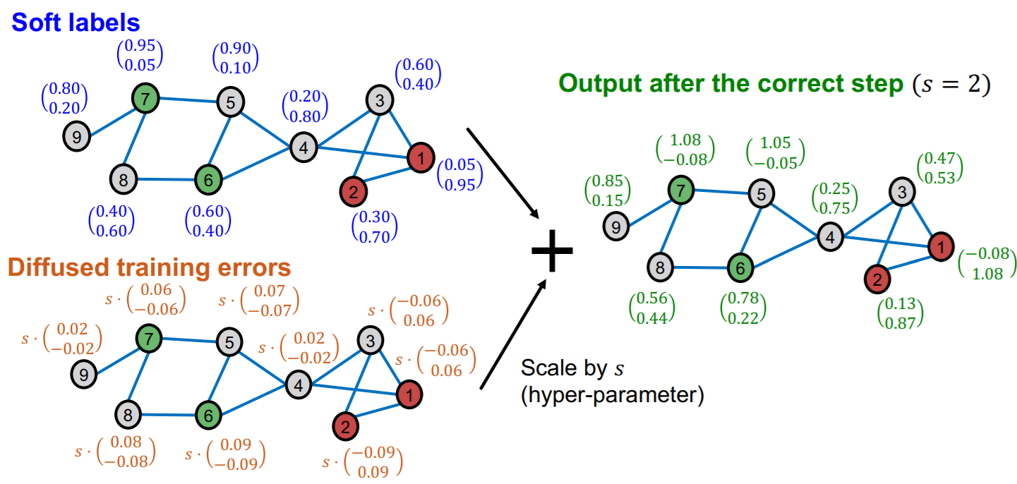
Correct step

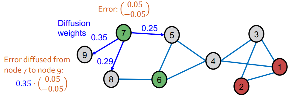
Idea

• error in one node \(\rightarrow\) similar error to its neighbors
• thus, spread an uncertainty!

[Step 1] compute “training errors”

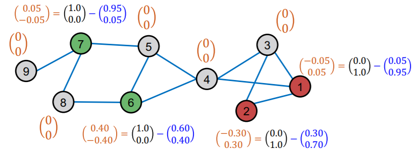
[Step 2] diffuse “training errors” \(\boldsymbol{E}^{(0)}\) along edges

• \(\boldsymbol{E}^{(0)}\) : initial training error matrix

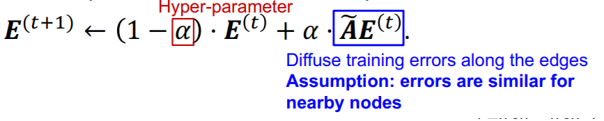
• \(\boldsymbol{A}\) : adjacency matrix
  • add self-loop ( \(A_{ii} =1\) )
• \(\tilde{\boldsymbol{A}}\) : diffusion matrix
  • \(\widetilde{\boldsymbol{A}} \equiv \boldsymbol{D}^{-1 / 2} \boldsymbol{A D}^{-1 / 2}\).
    • \(\mathbf{D}\) : degree matrix

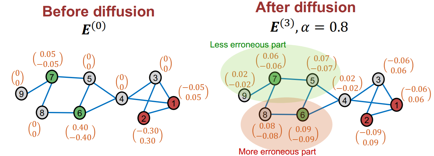
After diffusion…

More about \(\tilde{\boldsymbol{A}}\)

• “NORMALIZED” diffusion matrix
• all eigenvalues \(\lambda\)s are in [-1,1]
• \(\tilde{\boldsymbol{A}}^K\) ‘s eigenvalues \(\lambda\)s are also in [-1,1]

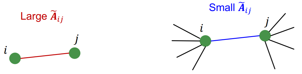
Intuition

• if \(i\) & \(j\) are connected…\(\widetilde{\boldsymbol{A}}_{i j} = \frac{1}{\sqrt{d_{i}} \sqrt{d_{j}}}\).
  • if large : connected ONLY with each other
  • if small : connected ALSO with others

[Step 3] add diffusion error to predicted value

• scale diffusion error ( \(s\) )

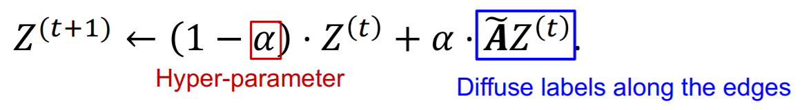
Smooth step

Idea :

• Neighboring nodes tend to share the same labels
• for LABELED nodes…use “hard” (soft (X)) labels

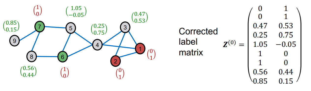
Smoothing procedure

• diffuse label \(\mathbf{Z}^{(0)}\)

  ( where \(\mathbf{Z}^{(0)}\) is “corrected label matrix” )

Result

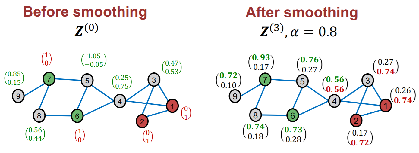
• final classification : argmax!