Pytorch Geometric Temporal

( 참고 : https://www.youtube.com/watch?v=Rws9mf1aWUs&list=PLV8yxwGOxvvoNkzPfCx2i8an–Tkt7O8Z&index=19)

Install Packages
Load Dataset
Data Introduction
Train & Test Split
Model ( A3TGCN )
Training
Evaluation

1. Install Packages

( 패키지 설치에 시간이 좀 걸린다…! )

import torch
from IPython.display import clear_output
pt_version = torch.__version__

!pip install torch-scatter -f https://pytorch-geometric.com/whl/torch-${pt_version}.html
!pip install torch-sparse -f https://pytorch-geometric.com/whl/torch-${pt_version}.html
!pip install torch-cluster -f https://pytorch-geometric.com/whl/torch-${pt_version}.html
!pip install torch-spline-conv -f https://pytorch-geometric.com/whl/torch-${pt_version}.html
!pip install torch-geometric
!pip install torch-geometric-temporal
clear_output()

2. Load Dataset

데이터셋 : METRLADatasetLoader

from torch_geometric_temporal.dataset import METRLADatasetLoader
loader = METRLADatasetLoader()
dataset = loader.get_dataset(num_timesteps_in=12, num_timesteps_out=12)

print("Dataset type:  ", dataset)
print("Number of samples / sequences: ",  len(set(dataset)))

Dataset type:   <torch_geometric_temporal.signal.static_graph_temporal_signal.StaticGraphTemporalSignal object at 0x7fb1f73fae50>
Number of samples / sequences:  34249

list(set(dataset))[0:5]

[Data(x=[207, 2, 12], edge_index=[2, 1722], edge_attr=[1722], y=[207, 12]),
 Data(x=[207, 2, 12], edge_index=[2, 1722], edge_attr=[1722], y=[207, 12]),
 Data(x=[207, 2, 12], edge_index=[2, 1722], edge_attr=[1722], y=[207, 12]),
 Data(x=[207, 2, 12], edge_index=[2, 1722], edge_attr=[1722], y=[207, 12]),
 Data(x=[207, 2, 12], edge_index=[2, 1722], edge_attr=[1722], y=[207, 12])]

3. Data Introduction

Traffic Forecasting 데이터

시계열의 개수 : 207개의 node ( loop detectors / sensors )
- 각 시계열은 2차원 ( speed & time )
기간 : 2012/3 ~ 2012/6
출처 : DCRNN

print("Dataset type:  ", dataset)
print("Number of samples / sequences: ",  len(set(dataset)))

Dataset type:   <torch_geometric_temporal.signal.static_graph_temporal_signal.StaticGraphTemporalSignal object at 0x7f56400dc890>
Number of samples / sequences:  34249

next(iter(dataset))

Data(x=[207, 2, 12], edge_index=[2, 1722], edge_attr=[1722], y=[207, 12])

x=[207, 2, 12]

207 : 시계열 개수
2 : 데이터 차원 ( speed & time )
12 : 과거 1시간을 window로 삼음 ( 60분/5분 = 12 )

edge_index=[2, 1722]

총 1722개의 엣지

edge_attr=[1722]

1차원 (scalar) 의 엣지 특성

y=[207, 12]

향후 1시간 ( 60/5=12 )에 대한 예측을 수행해야!

data_idx = 12345
sensor_idx = 77

sample_data = list(dataset)[data_idx]
print(sample_data.y)
print(sample_data.y[sensor_idx]) 

tensor([[0.7002, 0.7070, 0.6445,  ..., 0.5394, 0.5641, 0.6074],
        [0.2425, 0.5971, 0.5888,  ..., 0.6631, 0.3277, 0.6259],
        [0.2981, 0.6851, 0.6569,  ..., 0.7373, 0.7015, 0.7311],
        ...,
        [0.5517, 0.5036, 0.6754,  ..., 0.5579, 0.1957, 0.4775],
        [0.7682, 0.7345, 0.7249,  ..., 0.7125, 0.7400, 0.6754],
        [0.5146, 0.3992, 0.4899,  ..., 0.4033, 0.1133, 0.3600]])
tensor([0.5394, 0.5256, 0.5888, 0.6356, 0.6631, 0.7064, 0.5971, 0.6905, 0.6940,
        0.6012, 0.5366, 0.5703])

1일 치의 데이터 ( 24시간 )

hours = 24
list(dataset)[:hours]

[Data(x=[207, 2, 12], edge_index=[2, 1722], edge_attr=[1722], y=[207, 12]),
 Data(x=[207, 2, 12], edge_index=[2, 1722], edge_attr=[1722], y=[207, 12]),
 Data(x=[207, 2, 12], edge_index=[2, 1722], edge_attr=[1722], y=[207, 12]),
 Data(x=[207, 2, 12], edge_index=[2, 1722], edge_attr=[1722], y=[207, 12]),
 Data(x=[207, 2, 12], edge_index=[2, 1722], edge_attr=[1722], y=[207, 12]),
 Data(x=[207, 2, 12], edge_index=[2, 1722], edge_attr=[1722], y=[207, 12]),
 Data(x=[207, 2, 12], edge_index=[2, 1722], edge_attr=[1722], y=[207, 12]),
 Data(x=[207, 2, 12], edge_index=[2, 1722], edge_attr=[1722], y=[207, 12]),
 Data(x=[207, 2, 12], edge_index=[2, 1722], edge_attr=[1722], y=[207, 12]),
 Data(x=[207, 2, 12], edge_index=[2, 1722], edge_attr=[1722], y=[207, 12]),
 Data(x=[207, 2, 12], edge_index=[2, 1722], edge_attr=[1722], y=[207, 12]),
 Data(x=[207, 2, 12], edge_index=[2, 1722], edge_attr=[1722], y=[207, 12]),
 Data(x=[207, 2, 12], edge_index=[2, 1722], edge_attr=[1722], y=[207, 12]),
 Data(x=[207, 2, 12], edge_index=[2, 1722], edge_attr=[1722], y=[207, 12]),
 Data(x=[207, 2, 12], edge_index=[2, 1722], edge_attr=[1722], y=[207, 12]),
 Data(x=[207, 2, 12], edge_index=[2, 1722], edge_attr=[1722], y=[207, 12]),
 Data(x=[207, 2, 12], edge_index=[2, 1722], edge_attr=[1722], y=[207, 12]),
 Data(x=[207, 2, 12], edge_index=[2, 1722], edge_attr=[1722], y=[207, 12]),
 Data(x=[207, 2, 12], edge_index=[2, 1722], edge_attr=[1722], y=[207, 12]),
 Data(x=[207, 2, 12], edge_index=[2, 1722], edge_attr=[1722], y=[207, 12]),
 Data(x=[207, 2, 12], edge_index=[2, 1722], edge_attr=[1722], y=[207, 12]),
 Data(x=[207, 2, 12], edge_index=[2, 1722], edge_attr=[1722], y=[207, 12]),
 Data(x=[207, 2, 12], edge_index=[2, 1722], edge_attr=[1722], y=[207, 12]),
 Data(x=[207, 2, 12], edge_index=[2, 1722], edge_attr=[1722], y=[207, 12])]

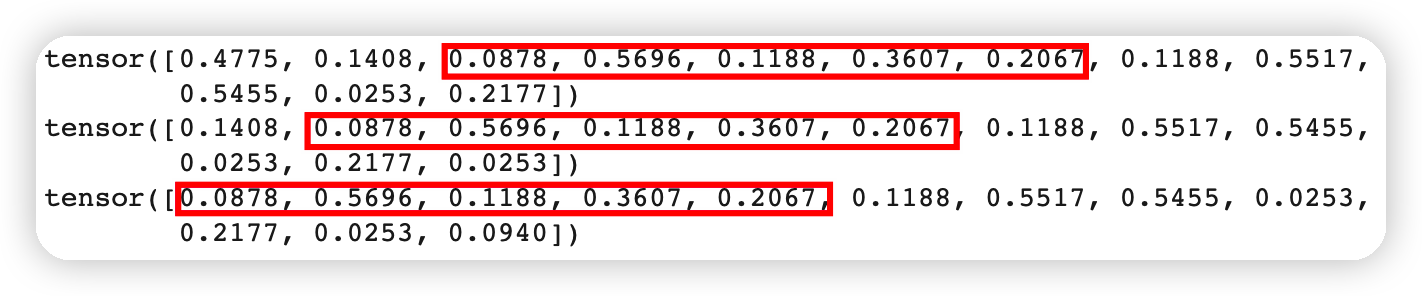
5분 간격 (데이터 1개 단위)로, 서로 밀려있음을 알 수 있다

hour1 = 0
hour2 = 1
hour3 = 2

bucket1 = list(dataset)[hour1]
bucket2 = list(dataset)[hour2]
bucket3 = list(dataset)[hour3]

sensor_idx = 77

print(bucket1.y[sensor_idx])
print(bucket2.y[sensor_idx])
print(bucket3.y[sensor_idx])

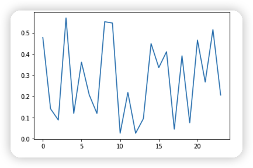
하나의 시계열 ( 하나의 sensor ) 데이터를 들여다보자.

import seaborn as sns

sensor_idx = 77
hours = 24

sensor_labels = [bucket.y[sensor_idx][0].item() for bucket in list(dataset)[:hours]]
sns.lineplot(data=sensor_labels)

4. Train & Test Split

from torch_geometric_temporal.signal import temporal_signal_split
train_dataset, test_dataset = temporal_signal_split(dataset, train_ratio=0.8)

print("Number of train buckets: ", len(set(train_dataset)))
print("Number of test buckets: ", len(set(test_dataset)))

Number of train buckets:  27399
Number of test buckets:  6850

5. Model ( A3TGCN )

import torch
import torch.nn.functional as F
from torch_geometric_temporal.nn.recurrent import A3TGCN

class TemporalGNN(torch.nn.Module):
    def __init__(self, node_features, input_periods, output_periods):
        super(TemporalGNN, self).__init__()
        # node_features = 2 ( speed & time )
        # periods = 12 ( 향후 12 step을 예측 )
        self.tgnn = A3TGCN(in_channels=node_features, 
                           out_channels=32, 
                           periods=input_periods)
        # single-shot prediction
        self.linear = torch.nn.Linear(32, output_periods)

    def forward(self, x, edge_index):
      	# x 크기 : (207, 2, 12)
        # edge_index 크기 : (2, 1722)
        h = self.tgnn(x, edge_index)
        # h 크기 : (207, 32)
        h = F.relu(h)
        h = self.linear(h)
        # h 크기 : (207, 12)
        return h

TemporalGNN(node_features=2, 
            input_periods=12,
            output_periods=12)

TemporalGNN(
  (tgnn): A3TGCN(
    (_base_tgcn): TGCN(
      (conv_z): GCNConv(2, 32)
      (linear_z): Linear(in_features=64, out_features=32, bias=True)
      (conv_r): GCNConv(2, 32)
      (linear_r): Linear(in_features=64, out_features=32, bias=True)
      (conv_h): GCNConv(2, 32)
      (linear_h): Linear(in_features=64, out_features=32, bias=True)
    )
  )
  (linear): Linear(in_features=32, out_features=12, bias=True)
)

6. Training

device = torch.device('cpu')
model = TemporalGNN(node_features=2, periods=12).to(device)
optimizer = torch.optim.Adam(model.parameters(), lr=0.01)

break_step = 2000

model.train()
print("Running training...")
for epoch in range(10): 
    loss = 0
    step = 0
    for data in train_dataset:
      	#----------------------------------#
        data = data.to(device)
        X = data.x
        E = data.edge_index
        y = data.y
        #----------------------------------#
        y_hat = model(X,E) # (207, 12)
        #----------------------------------#
        loss += torch.mean((y_hat - y)**2) 
        step += 1
        if step > break_step:
          break

    loss = loss / (step + 1)
    loss.backward()
    optimizer.step()
    optimizer.zero_grad()
    print("Epoch {} train MSE: {:.4f}".format(epoch, loss.item()))

Running training...
Epoch 0 train MSE: 0.7586
Epoch 1 train MSE: 0.7382
Epoch 2 train MSE: 0.7172
Epoch 3 train MSE: 0.6940
Epoch 4 train MSE: 0.6688
Epoch 5 train MSE: 0.6429
Epoch 6 train MSE: 0.6183
Epoch 7 train MSE: 0.5974
Epoch 8 train MSE: 0.5817
Epoch 9 train MSE: 0.5693

7. Evaluation

하루(1일) 만큼 예측을 진행한다.

model.eval()
loss = 0
step = 0
horizon = 288 # 1일 = 24시간 = 24x12개의 "5분"

y_labels = []
y_labels = []

for data in test_dataset:
  	#----------------------------------#
    data = data.to(device)
    X = data.x
    E = data.edge_index
    y = data.y
    #----------------------------------#
    y_hat = model(X,E)
    loss += torch.mean((y_hat - y)**2)
    #----------------------------------#
    y_labels.append(y)
    y_labels.append(y_hat)
    #----------------------------------#
    step += 1
    if step > horizon:
          break

loss = loss / (step+1)
loss = loss.item()
print("Test MSE: {:.4f}".format(loss))

Test MSE: 0.6862

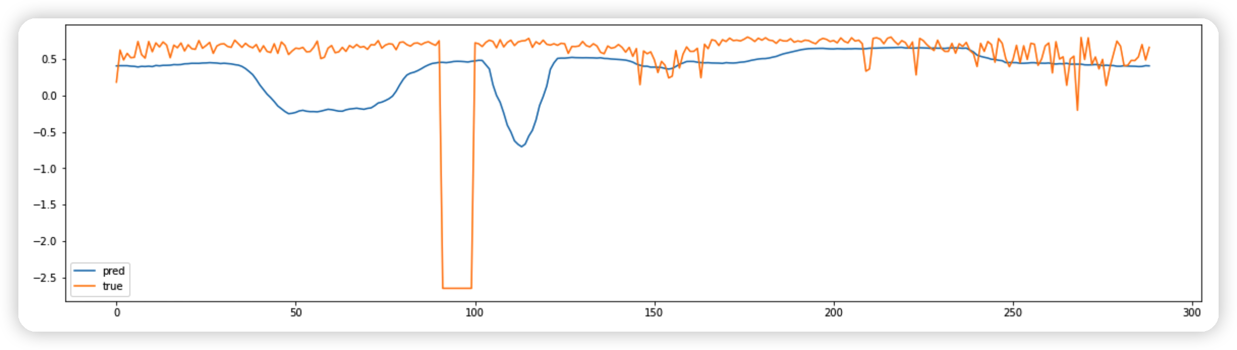
8. Visualization

prediction 크기 :

207 : 시계열(센서) 개수
12 : 미래 예측 길이

import numpy as np

sensor = 123
timestep = 11 
preds = np.asarray([pred[sensor][timestep].detach().cpu().numpy() for pred in predictions])
labs  = np.asarray([label[sensor][timestep].cpu().numpy() for label in labels])
print("Data points:,", preds.shape)

Data points:, (289,)

import matplotlib.pyplot as plt 
plt.figure(figsize=(20,5))
sns.lineplot(data=preds, label="pred")
sns.lineplot(data=labs, label="true")

Twitter Facebook LinkedIn

(PyG) Pytorch Geometric Temporal

Seunghan Lee