( Skip the basic parts + not important contents )

11.Sampling MethodsPermalink

For most probabilsitic models, exact inference is INTRACTABLE!

$\rightarrow$ Ch11 : approximate inference based on numerical sampling, known as Monte Carlo techniques

Goal : evaluate $\mathbb{E}[f]=\int f(\mathbf{z}) p(\mathbf{z}) \mathrm{d} \mathbf{z}$

• using finite sum : $\widehat{f}=\frac{1}{L} \sum_{l=1}^{L} f\left(\mathbf{z}^{(l)}\right)$
• variance of the estimator : $\operatorname{var}[\widehat{f}]=\frac{1}{L} \mathbb{E}\left[(f-\mathbb{E}[f])^{2}\right]$

However, samples $\mathbf{z}^{(l)}$ may not be independent!

( thus, effective sample size might be much smaller than the apparent sample size )

11-1. Basic Sampling AlgorithmsPermalink

11-1-1. Standard distributionsPermalink

skip

11-1-2. Rejection SamplingPermalink

sample from complex distn

wish to sample from $p(z)$, which $p(z)=\frac{1}{Z_{p}} \widetilde{p}(z)$

• sampling is hard
• evaluation is easy

1) use “proposal distribution” $q(z)$

• more simple distribution

2) introduce constant $k$

• where $k q(z) \geqslant \widetilde{p}(z)$
• $k q(z)$ : comparison function

Algorithm

• [step 1] generate $z_0$ from $q(z)$

• [step 2] generate $u_0$ from $\text{Unif}(0,kq(z_0))$

• [step 3] if $u_{0}>\widetilde{p}\left(z_{0}\right)$ : reject

  ( o.w : accept )

11-1-3. Adaptive rejection samplingPermalink

skip

11-1-4. Importance samplingPermalink

Finite sum approximation to expectation

(1) discrete $z$ space into a uniform grid

(2) evaluate the integrand as a sum : $\mathbb{E}[f] \simeq \sum_{l=1}^{L} p\left(\mathbf{z}^{(l)}\right) f\left(\mathbf{z}^{(l)}\right)$.

Problem : summation grows exponentially with the dim of $z$

Normalized casePermalink

finite sum over samples $\left\{\mathbf{z}^{(l)}\right\}$ drawn from $q(\mathbf{z})$ :

$\begin{aligned} \mathbb{E}[f] &=\int f(\mathbf{z}) p(\mathbf{z}) \mathrm{d} \mathbf{z} \\ &=\int f(\mathbf{z}) \frac{p(\mathbf{z})}{q(\mathbf{z})} q(\mathbf{z}) \mathrm{d} \mathbf{z} \\ & \simeq \frac{1}{L} \sum_{l=1}^{L} \frac{p\left(\mathbf{z}^{(l)}\right)}{q\left(\mathbf{z}^{(l)}\right)} f\left(\mathbf{z}^{(l)}\right) \end{aligned}$.

we call $r_{l}=p\left(\mathbf{z}^{(l)}\right) / q\left(\mathbf{z}^{(l)}\right)$, importance weights

Unnormalized casePermalink

$p(\mathrm{z})$ can only be evaluated up to a normalization constant

( $p(\mathrm{z})=\widetilde{p}(\mathrm{z}) / Z_{p}$ )

$\begin{aligned} \mathbb{E}[f] &=\int f(\mathbf{z}) p(\mathbf{z}) \mathrm{d} \mathbf{z} \\ &=\frac{Z_{q}}{Z_{p}} \int f(\mathbf{z}) \frac{\widetilde{p}(\mathbf{z})}{\widetilde{q}(\mathbf{z})} q(\mathbf{z}) \mathrm{d} \mathbf{z} \\ & \simeq \frac{Z_{q}}{Z_{p}} \frac{1}{L} \sum_{l=1}^{L} \widetilde{r}_{l} f\left(\mathbf{z}^{(l)}\right) \end{aligned}$.

where $\tilde{r}_{l}=\tilde{p}\left(\mathbf{z}^{(l)}\right) / \widetilde{q}\left(\mathbf{z}^{(l)}\right) .$

since $\begin{aligned} \frac{Z_{p}}{Z_{q}} &=\frac{1}{Z_{q}} \int \tilde{p}(\mathbf{z}) \mathrm{d} \mathbf{z}=\int \frac{\tilde{p}(\mathbf{z})}{\widetilde{q}(\mathbf{z})} q(\mathbf{z}) \mathrm{d} \mathbf{z} \simeq \frac{1}{L} \sum_{l=1}^{L} \widetilde{r}_{l} \end{aligned}$

$\mathbb{E}[f] \simeq \sum_{l=1}^{L} w_{l} f\left(\mathbf{z}^{(l)}\right)$, where $w_{l}=\frac{\tilde{r}_{l}}{\sum_{m} \tilde{r}_{m}}=\frac{\tilde{p}\left(\mathbf{z}^{(l)}\right) / q\left(\mathbf{z}^{(l)}\right)}{\sum_{m} \tilde{p}\left(\mathbf{z}^{(m)}\right) / q\left(\mathbf{z}^{(m)}\right)}$

11-1-5. Sampling-importance-resamplingPermalink

skip

11-1-6. Sampling and the EM algorithmPermalink

skip

11-2. MCMCPermalink

Metropolis algorithmPermalink

• when proposal distribution is symmetric
• acceptance probability : $A\left(\mathrm{z}^{\star}, \mathrm{z}^{(\tau)}\right)=\min \left(1, \frac{\tilde{p}\left(\mathrm{z}^{\star}\right)}{\widetilde{p}\left(\mathrm{z}^{(\tau)}\right)}\right)$.

Metropolis Hastings algorithmPermalink

• when proposal distribution does not need to be symmetric

• acceptance probability : $A_{k}\left(\mathrm{z}^{\star}, \mathrm{z}^{(\tau)}\right)=\min \left(1, \frac{\tilde{p}\left(\mathrm{z}^{\star}\right) q_{k}\left(\mathrm{z}^{(\tau)} \mid \mathrm{z}^{\star}\right)}{\tilde{p}\left(\mathrm{z}^{(\tau)}\right) q_{k}\left(\mathrm{z}^{\star} \mid \mathrm{z}^{(\tau)}\right)}\right)$

• pf) detailed balance is satisfied!

  $\begin{aligned} p(\mathbf{z}) q_{k}\left(\mathbf{z} \mid \mathbf{z}^{\prime}\right) A_{k}\left(\mathbf{z}^{\prime}, \mathbf{z}\right) &=\min \left(p(\mathbf{z}) q_{k}\left(\mathbf{z} \mid \mathbf{z}^{\prime}\right), p\left(\mathbf{z}^{\prime}\right) q_{k}\left(\mathbf{z}^{\prime} \mid \mathbf{z}\right)\right) \\ &=\min \left(p\left(\mathbf{z}^{\prime}\right) q_{k}\left(\mathbf{z}^{\prime} \mid \mathbf{z}\right), p(\mathbf{z}) q_{k}\left(\mathbf{z} \mid \mathbf{z}^{\prime}\right)\right) \\ &=p\left(\mathbf{z}^{\prime}\right) q_{k}\left(\mathbf{z}^{\prime} \mid \mathbf{z}\right) A_{k}\left(\mathbf{z}, \mathbf{z}^{\prime}\right) \end{aligned}$.

11-3. Gibbs samplingPermalink

1. Initialize $\left\{z_{i}: i=1, \ldots, M\right\}$
2. For $\tau=1, \ldots, T:$ $-$ Sample $z_{1}^{(\tau+1)} \sim p\left(z_{1} \mid z_{2}^{(\tau)}, z_{3}^{(\tau)}, \ldots, z_{M}^{(\tau)}\right)$ $-$ Sample $z_{2}^{(\tau+1)} \sim p\left(z_{2} \mid z_{1}^{(\tau+1)}, z_{3}^{(\tau)}, \ldots, z_{M}^{(\tau)}\right)$ : $-$ Sample $z_{j}^{(\tau+1)} \sim p\left(z_{j} \mid z_{1}^{(\tau+1)}, \ldots, z_{j-1}^{(\tau+1)}, z_{j+1}^{(\tau)}, \ldots, z_{M}^{(\tau)}\right)$ : Sample $z_{M}^{(\tau+1)} \sim p\left(z_{M} \mid z_{1}^{(\tau+1)}, z_{2}^{(\tau+1)}, \ldots, z_{M-1}^{(\tau+1)}\right)$

Acceptance ratio = (always) 1

pf) $A\left(\mathrm{z}^{\star}, \mathrm{z}\right)=\frac{p\left(\mathrm{z}^{\star}\right) q_{k}\left(\mathrm{z} \mid \mathrm{z}^{\star}\right)}{p(\mathrm{z}) q_{k}\left(\mathrm{z}^{\star} \mid \mathrm{z}\right)}=\frac{p\left(z_{k}^{\star} \mid \mathrm{z}_{\backslash k}^{\star}\right) p\left(\mathrm{z}_{\backslash k}^{\star}\right) p\left(z_{k} \mid \mathrm{z}_{\backslash k}^{\star}\right)}{p\left(z_{k} \mid \mathrm{z} \backslash k\right) p(\mathrm{z} \backslash k) p\left(z_{k}^{\star} \mid \mathrm{z} \backslash k\right)}=1$

11-4. Slice SamplingPermalink

difficulties of Metropolis : “sensitive to step size”

• too small : slow decorrelation
• too large : inefficiency due to high rejection rate

Slice sampling : provides an “adaptive step size”

Involves augmenting $z$ with an additional variable $u$

then, draw samples from joint $(z,u)$ space

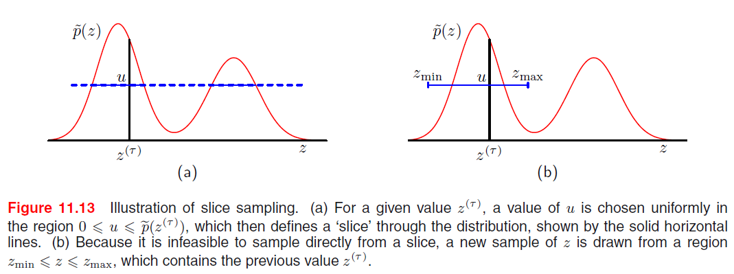
Goal : sample from $\hat{p}(z, u)=\left\{\begin{array}{ll} 1 / Z_{p} & \text { if } 0 \leqslant u \leqslant \tilde{p}(z) \\ 0 & \text { otherwise } \end{array}\right.$

where $Z_{p}=\int \tilde{p}(z) \mathrm{d} z .$

It is okay to sample from $\hat{p}(z, u)$ and then just discard $u$

$\int \hat{p}(z, u) \mathrm{d} u=\int_{0}^{\widetilde{p}(z)} \frac{1}{Z_{p}} \mathrm{~d} u=\frac{\tilde{p}(z)}{Z_{p}}=p(z)$.

Algorithm : alternately sample $z$ and $u$

• step 1) given $z$, evaluate $\tilde{p(z)}$
• step 2) sample $u$ from $\text{Unif}(0,\tilde{p(z)})$
• step 3) fix $u$ and sample $z$ , distribution defined by $\{z: \tilde{p}(z)>u\}$

11-5. The Hybrid MC algorithmPermalink

limitation of Metropolis : “random walk”

introduce a sophisticated class of transition, based on physical system

Applicable to..

• distributions over continuous variables
• for which we can readily evaluate the gradient of log probability w.r.t state variable

11-5-1. Dynamic SystemsPermalink

dynamics : $\tau$

state variable : $z$

momentum variable : $r$

$r_{i}=\frac{\mathrm{d} z_{i}}{\mathrm{~d} \tau}$.

Hamiltonian function $H$ : $H(\mathbf{z}, \mathbf{r})=E(\mathbf{z})+K(\mathbf{r})$

• $p(\mathbf{z})=\frac{1}{Z_{p}} \exp (-E(\mathbf{z}))$.
  • $E(\mathbf{z})$ : potential energy
• $K(\mathbf{r})=\frac{1}{2}\|\mathbf{r}\|^{2}=\frac{1}{2} \sum_{i} r_{i}^{2}$.
  • kinetic energy

Hamiltonian Equation

• $\begin{aligned} \frac{\mathrm{d} z_{i}}{\mathrm{~d} \tau} &=\frac{\partial H}{\partial r_{i}} \\ \frac{\mathrm{d} r_{i}}{\mathrm{~d} \tau} &=-\frac{\partial H}{\partial z_{i}} \end{aligned}$.

Properties

• 1) during the evolution of this dynamical system $H$ is constant

  $\begin{aligned} \frac{\mathrm{d} H}{\mathrm{~d} \tau} &=\sum_{i}\left\{\frac{\partial H}{\partial z_{i}} \frac{\mathrm{d} z_{i}}{\mathrm{~d} \tau}+\frac{\partial H}{\partial r_{i}} \frac{\mathrm{d} r_{i}}{\mathrm{~d} \tau}\right\} \\ &=\sum_{i}\left\{\frac{\partial H}{\partial z_{i}} \frac{\partial H}{\partial r_{i}}-\frac{\partial H}{\partial r_{i}} \frac{\partial H}{\partial z_{i}}\right\}=0 \end{aligned}$.

• 2) Liouville’s Theorem : preserve volume in phase space

  $$\mathbf{V}=\left(\frac{\mathrm{d} \mathbf{z}}{\mathrm{d} \tau}, \frac{\mathrm{d} \mathbf{r}}{\mathrm{d} \tau}\right)$$

  $\begin{aligned} \operatorname{div} \mathbf{V} &=\sum_{i}\left\{\frac{\partial}{\partial z_{i}} \frac{\mathrm{d} z_{i}}{\mathrm{~d} \tau}+\frac{\partial}{\partial r_{i}} \frac{\mathrm{d} r_{i}}{\mathrm{~d} \tau}\right\} \\ &=\sum_{i}\left\{-\frac{\partial}{\partial z_{i}} \frac{\partial H}{\partial r_{i}}+\frac{\partial}{\partial r_{i}} \frac{\partial H}{\partial z_{i}}\right\}=0 \end{aligned}$.

Joint pdf

• total energy = Hamiiltonian
• $p(\mathbf{z}, \mathbf{r})=\frac{1}{Z_{H}} \exp (-H(\mathbf{z}, \mathbf{r}))$.

Due to 2 properties : Hamiltonian dynamics will leave $p(z,r)$ invariant

• volume of this region will remain unchanged
• thus, $H$, and probability density will remain unchanged

Althoough $H$ is invariant, $z$ and $r$ will vary

In order to arrive at an ergodic sampling…

$\rightarrow$ introduce additional moves

$\rightarrow$ change the value of $H$ while leaving $p(z,r)$ unchanged!

By “replacing $z$ with one drawn from its distribution conditioned on $z$ “

( $z$ and $r$ are independent in $p(z,r)$, so conditional $p(r\mid z)$ is a Gaussian )

Leapfrog discretizationPermalink

successive updates to position ($z$) and momentum $(r)$

• time interval : $\tau$ $\rightarrow$ need $\tau/\epsilon$ steps

SummaryPermalink

Hamiltonian dynamical approach invloves alternating between

• series of leapfrog updates
• re-sampling of the momentum variables

Unlike Metropolis, able to make use of “gradient of log prob”

11-5-2. Hybrid MCPermalink

Hybrid MC = Hamiltonian dynamics + Metropolis

After each application of leapfrog…

• resulting candidate state is ACCEPTED/REJECTED according to the Metropolis criterion

  ( based on the value of Hamiltonian $H$ )

  $\min \left(1, \exp \left\{H(\mathbf{z}, \mathbf{r})-H\left(\mathbf{z}^{\star}, \mathbf{r}^{\star}\right)\right\}\right)$.

• perfect : $H$ unchanged $\rightarrow$ 100% accept

• numerical errors : $H$ may sometimes decrease