(Pytorch) 05.Monte Carlo Drop Out (MCDO)

Monte Carlo Drop Out (MCDO)

( 이론 참고 : https://seunghan96.github.io/bnn/17.Dropout-as-Bayesian-Approximation-(2016)/)

( 코드 참고 : https://github.com/cpark321/uncertainty-deep-learning/ )

1. Import Packages

import numpy as np
from matplotlib import pyplot as plt
import seaborn as sns
import torch
import torch.nn as nn
import torch.nn.functional as F
import torch.optim as optim

device = torch.device("cuda:0" if torch.cuda.is_available() else "cpu")

2. Make Sample Dataset

(1) 임의의 가상 dataset을 만든다 ( n =10000 )

• Y_real : \(f(x)\)
• Y_noise : \(f(x)\) + \(\epsilon\), where \(\epsilon \sim N(0,1^2)\)

def func(x):
    return -0.8*np.power(x, 3)+2*np.power(x, 2)+4*x

n=10000
sigma=1

X = np.linspace(-3, 3, n)
Y_real = func(X)
Y_noise = (Y_real+np.random.normal(0,sigma,n))

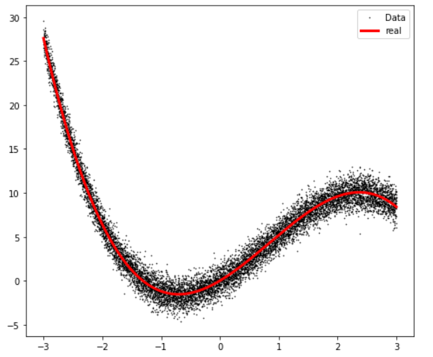
(2) data의 분포

plt.rcParams['figure.figsize'] = [8, 7]
plt.plot(X, Y_noise, '.', markersize=1, color='black')
plt.plot(X, Y_real, 'r', linewidth=3,color='red')
plt.legend(['Data', 'y=x^3'], loc = 'best')
plt.show()

(3) shape 변경

X = X.reshape(-1, 1)
Y_noise = Y_noise.reshape(-1, 1)

(4) Scaling ( 표준정규분포로 )

• X와 Y를 모두 scale해준다.

from sklearn.preprocessing import StandardScaler
x_scaler = StandardScaler()
y_scaler = StandardScaler()
X_scaled = x_scaler.fit_transform(X)
Y_noise_scaled = y_scaler.fit_transform(Y_noise)

3. Modeling

• 3-1 ) 여러 layer를 쌓는 함수 : make_sequential
• 3-2 ) 기본 Network : BaseModel

3-1. 여러 layer를 쌓는 함수 : make_sequential

dropout을 가진 layer들을 쌓는다. 아래와 같이 3가지를 지정해준다

• input dimension
• output dimension
• dropout rate

def make_sequential(in_,out_,do_rate):
    return nn.Sequential(nn.Linear(in_,out_),
                       nn.ReLU(),
                       nn.Dropout(p=do_rate))

3-2. 기본 Network : BaseModel

class BaseModel(nn.Module):
  def __init__(self,input_dim,hidden_dim,output_dim,
               hidden_L,do_rate,w_decay):
    super(BaseModel,self).__init__()
    self.input_dim = input_dim
    self.output_dim = output_dim
    self.do_rate = do_rate
    self.w_decay = w_decay
    self.in_layer = nn.Linear(input_dim,hidden_dim)
    
    self.layers = nn.ModuleList()
    self.layers.append(make_sequential(input_dim,hidden_dim,self.do_rate))
    self.layers.extend([make_sequential(hidden_dim,hidden_dim,self.do_rate) for _ in range(hidden_L)])
    self.layers.append(nn.Linear(hidden_dim,output_dim))


  def forward(self,x):
    for layer in self.layers:
      x = layer(x.float())
    return x.float()

4. Train Model

위에서 scaling된 데이터를, tensor 형태로 변환시켜서 모델에 넣는다.

X_scaled = torch.tensor(X_scaled,dtype=torch.float64).view(-1,1).to(device)
Y_noise_scaled = torch.tensor(Y_noise_scaled,dtype=torch.float64).view(-1,1).to(device)

모델을 학습시킨다

• optimizer : SGD
• loss function : Mean squared Error
• dropout rate : 0.2

model = BaseModel(input_dim=1,hidden_dim=20,output_dim=1,hidden_L=2,
                  do_rate=0.2,w_decay=1e-6).to(device)
loss_fn  = torch.nn.MSELoss()
optimizer = torch.optim.SGD(model.parameters(),lr=0.01,weight_decay=model.w_decay)

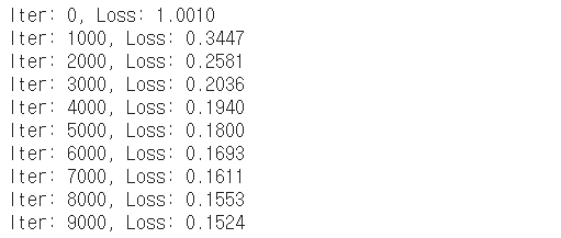
for iter in range(10000):
    Y_pred_scaled = model(X_scaled).float()
    optimizer.zero_grad()
    loss = loss_fn(Y_pred_scaled,Y_noise_scaled.float())
    loss.backward()
    optimizer.step()
    
    if iter % 1000 == 0:
        print("Iter: {}, Loss: {:.4f}".format(iter, loss.item()))

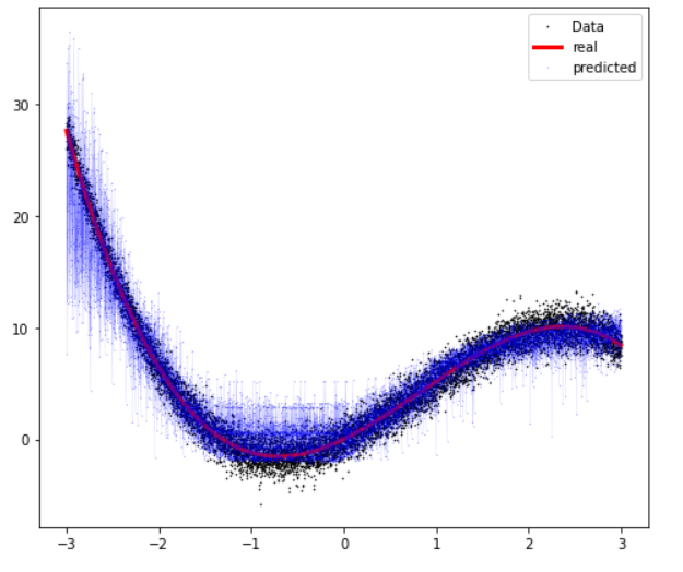
5. Result

예측된 Y값들을, 다시 scaler를 사용해서 원래의 scale로 inverse transform한다

Y_pred =  y_scaler.inverse_transform(Y_pred_scaled.cpu().data.numpy())

Visualization

plt.rcParams['figure.figsize'] = [8, 7]
plt.plot(X, Y_noise, '.', markersize=1, color='black')
plt.plot(X, Y_real, 'r', linewidth=3,color='red')
plt.plot(X, Y_pred, '.', markersize=0.2,color='blue')
plt.plot(X, Y_pred, 'r', linewidth=0.05,color='blue')
plt.legend(['Data', 'real','predicted'], loc = 'best')
plt.show()

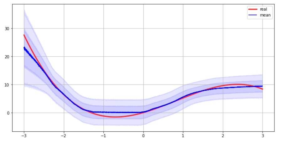
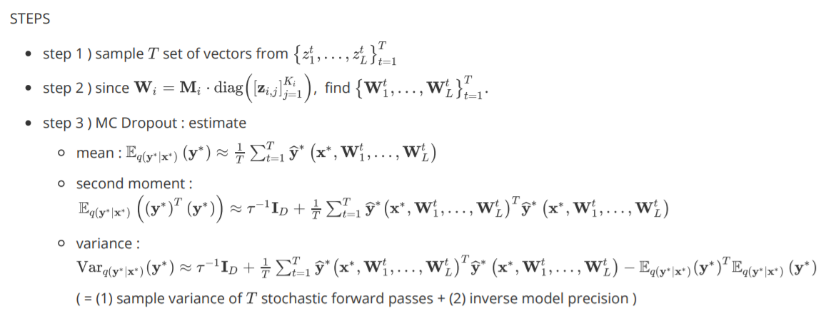
6. Uncertainty Estimation

해당 데이터로 총 1,000번 예측하여, 그 결과값들을 저장한다

해당 1,000개의 결과값으로

• mean
• variance

를 구한뒤, 시각적으로 uncertainty를 확인해본다.

def uncertainity_estimate(x, model, num_samples, l2):
    scaled_outputs = np.hstack([model(x).cpu().detach().numpy() for _ in range(num_samples)]) 
    outputs = y_scaler.inverse_transform(scaled_outputs)
    y_mean = outputs.mean(axis=1)
    y_variance = outputs.var(axis=1)
    tau = l2 * (1. - model.do_rate) / (2. * n * model.w_decay)
    y_variance += (1. / tau)
    y_std = np.sqrt(y_variance)

    return y_mean, y_std

y_mean,y_std = uncertainity_estimate(X_scaled,model,1000,0.01)

plt.figure(figsize=(12,6))
plt.plot(X, Y_real, ls="-", linewidth=3,color='red', alpha=0.8, label="real")
plt.plot(X, y_mean, ls="-", color="blue", label="mean")
for a in range(1,3):
    plt.fill_between(X.reshape(-1,),
        y_mean - y_std *a,
        y_mean + y_std *a,
        color="b",
        alpha=0.1)
plt.legend()
plt.grid()