Variational Auto Encoder
지난 포스트에서는 Variational Auto Encoder의 이론적인 부분에 대해서 다뤘다. 이번에는, 저번 시간에 배운 것을 Pytorch로 구현해보는 연습을 할 것이다.
( 참고 : https://github.com/bayesgroup/deepbayes-2019 )

https://theaisummer.com/assets/img/posts/vae.jpg
from torchvision.datasets import MNIST
from torchvision import transforms
import torch
from torch import nn
import numpy as np
import matplotlib.pylab as plt

torch.manual_seed(0)

if torch.cuda.is_available():
    device = torch.device('cuda:0')
else:
    device = torch.device('cpu')

print('Using torch version {}'.format(torch.__version__))
print('Using {} device'.format(device))
Using torch version 1.0.1
Using cpu device
실습에 사용할 데이터는 MNIST 손글씨 데이터이다.
# Training dataset
train_loader = torch.utils.data.DataLoader(
    MNIST(root='.', train=True, download=True,
          transform=transforms.ToTensor()),
    batch_size=100, shuffle=True, pin_memory=True)

# Test dataset
test_loader = torch.utils.data.DataLoader(
    MNIST(root='.', train=False, transform=transforms.ToTensor()),
    batch_size=100, shuffle=True, pin_memory=True)
1. Distributions for VAE
구현에 필요한 분포들을 불러온다 ( Normal & Bernoulli )
from torch.distributions import Normal, Bernoulli, Independent
2. Encoder & Decoder
Encoder와 Decoder를 다음과 같은 구조의 Neural Net으로 구성하였다.
D = 28*28 # 원본의 차원
d = 32 # 축소시키고자 하는 차원
nh = 100 # Layer 내의 Unit 개수

Encoder = nn.Sequential(
    nn.Linear(D, nh),
    nn.ReLU(),
    nn.Linear(nh, nh),
    nn.ReLU(),
    nn.Linear(nh, 2 * d))  # 2배인 이유 : mean의 d개 + variance의 d개

Decoder = nn.Sequential(
    nn.Linear(d, nh),
    nn.ReLU(),
    nn.Linear(nh, nh),
    nn.ReLU(),
    nn.Linear(nh, D)).to(device)

Encoder = Encoder.to(device)
Decoder = Decoder.to(device)
Encoder의 구조는 다음과 같다.
Encoder
Sequential(
  (0): Linear(in_features=784, out_features=100, bias=True)
  (1): ReLU()
  (2): Linear(in_features=100, out_features=100, bias=True)
  (3): ReLU()
  (4): Linear(in_features=100, out_features=64, bias=True)
)
Decoder의 구조는 다음과 같다.
Decoder
Sequential(
  (0): Linear(in_features=32, out_features=100, bias=True)
  (1): ReLU()
  (2): Linear(in_features=100, out_features=100, bias=True)
  (3): ReLU()
  (4): Linear(in_features=100, out_features=784, bias=True)
)
3. Loss Function
Encoder와 Decoder의 구현은 비교적 용이했다. 조금 더 복잡한 것은 바로 VAE의 Loss Function을 구현하는 것이었다. 저번 포스트에서 공부한 VAE의 Loss Function은 다음과 같았다.
\[\begin{align*} Loss(\phi, \theta) &= - \int q(Z \mid X, \phi)log \frac{p(X\mid Z, \theta)p(Z)}{q(Z\mid X,\phi)}dZ\\ &= - \int q(Z \mid X, \phi)log p(X\mid Z, \theta)dZ + KL(q(Z\mid X, \phi) \mid \mid p(Z)) \\ &= - \int q(Z \mid X, \phi)log p(X\mid Z, \theta)dZ - H(q(Z \mid X, \phi))+ H(q(Z\mid X, \phi),p(Z)) \end{align*}\\\]위의 Loss Function은 다음과 같이 크게 세 부분으로 구성되었다.
- PART 1 ) \(- \int q(Z \mid X, \phi)log p(X\mid Z, \theta)dZ\)
- Reconstruction Error
- \(X\) 에 대한 복원 오차
- Part 2 ) \(- H(q(Z \mid X, \phi))\)
- Posterior Entropy
- Posterior에서 샘플링 된 Z는 최대한 다양해야
- Part 3) \(H(q(Z\mid X, \phi),p(Z))\)
- Cross Entropy
- Posterior & Prior의 정보량은 유사해야
위의 Loss Function을 코드로 구현해볼 것이다
(1) Normal Distribution
구현하기에 앞서서, pytorch에서 Normal Distribution에서 sampling하는 함수는 다음과 같다.
normal_dist = Normal(loc=torch.zeros(10,3).to(device),scale=torch.ones(10,3).to(device))
iid_normal = Independent(normal_dist,reinterpreted_batch_ndims=1)
iid_normal.rsample()
tensor([[-1.7892, -1.0817,  1.6329],
        [ 0.7075, -0.8495,  2.0385],
        [-0.7659, -0.3014,  1.5344],
        [ 0.3087,  2.6570,  0.2698],
        [-1.4587, -0.7290, -0.9239],
        [-0.7545, -1.4928,  1.3577],
        [-1.5987, -0.4963, -1.7971],
        [ 0.8628, -0.8514, -1.7072],
        [-0.4711,  0.9973, -0.7414],
        [-0.1524,  0.2226,  0.7049]])
(2) Bernoulli Distribution
마찬가지로 Bernoulli Distribution도 다음과 같이 쉽게 사용할 수 있다.
bernoulli_dist = Bernoulli(logits=torch.FloatTensor(([5,3,1],
                                                     [1,2,3])).to(device))

iid_bernoulli = Independent(bernoulli_dist,reinterpreted_batch_ndims=1)
iid_bernoulli.log_prob(2)
tensor([8.6314, 5.5112])
(3) Define Loss Function
위에서 구현한 Encoder, Decoder, 그리고 loss function을 참고하여, (1) Loss와 (2) Decoder의 output을 출력하는 함수를 구현하였다.
def loss_fun(x,enc,dec):
    batch_size = x.size(0)

    ## (1) Encoder의 input : X -> latent vector (2d) 출력
    enc_output = enc(x)

    pz = Independent(Normal(loc = torch.zeros(batch_size,d).to(device), # mean
                           scale = torch.ones(batch_size,d).to(device)), # variance
                     reinterpreted_batch_ndims=1)
    qz_x = Independent(Normal(loc = enc_output[:,:d],
                             scale = torch.exp(enc_output[:,d:])),
                      reinterpreted_batch_ndims=1)

    ## (2) Decoder의 input : Z -> reconstruct
    z = qz_x.rsample()
    dec_output = dec(z)
    px_z = Independent(Bernoulli(logits=dec_output),
                      reinterpreted_batch_ndims=1)

    ## (3) Loss 계산
    loss = -(px_z.log_prob(x) + pz.log_prob(z) - qz_x.log_prob(z)).mean()

    return loss, dec_output
4. Training
학습을 위한 모든 준비는 끝났다. Optimizer로는 Adam Optimizer를 사용하였고, Training하는 함수는 다음과 같다.
from itertools import chain
def train_model(loss, model, batch_size=100, num_epochs=3, learning_rate=1e-3):

    #################### Optimizer 설정 ##########################
    gd = torch.optim.Adam(
        chain(*[x.parameters() for x in model
                if (isinstance(x, nn.Module) or isinstance(x, nn.Parameter))]),
        lr=learning_rate)

    #################### Training & Testing ########################
    train_losses = []
    test_results = []

    for _ in range(num_epochs):
        #### Train 단계 ####
        for i, (batch, _) in enumerate(train_loader):
            total = len(train_loader) # 총 batch의 개수
            gd.zero_grad()
            batch = batch.view(-1, D).to(device)
            loss_value, _ = loss(batch, *model) # Loss 계산
            loss_value.backward() # Back Propagation
            train_losses.append(loss_value.item())
            if (i + 1) % 50 == 0:
                print('\rTrain loss:', train_losses[-1],
                      'Batch', i + 1, 'of', total, ' ' * 10, end='', flush=True)
            gd.step()
        test_loss = 0.

        #### Test 단계 ####
        for i, (batch, _) in enumerate(test_loader):
            batch = batch.view(-1, D).to(device)
            batch_loss, _ = loss(batch, *model)
            test_loss += (batch_loss - test_loss) / (i + 1)
        print('\nTest loss after an epoch: {}'.format(test_loss))
train_model(loss_fun, model=[Encoder, Decoder], num_epochs=16)
Train loss: 209.75807189941406 Batch 50 of 600            203.1555633544922 Batch 100 of 600            199.5128173828125 Batch 150 of 600            202.78440856933594 Batch 200 of 600            192.7709503173828 Batch 250 of 600            194.23851013183594 Batch 300 of 600            192.98529052734375 Batch 350 of 600     ....
Test loss after an epoch: 111.55714416503906
Train loss: 106.00868225097656 Batch 50 of 600            109.53474426269531 Batch 100 of 600            112.19305419921875 Batch 150 of 600            112.34392547607422 Batch 200 of 600            112.25574493408203 Batch 250 of 600            115.48812866210938 Batch 300 of 600            115.19200134277344 Batch 350 of 600            115.97611999511719 Batch 400 of 600            113.45658874511719 Batch 450 of 600            117.41264343261719 Batch 500 of 600            107.6280288696289 Batch 550 of 600            113.7376480102539 Batch 600 of 600
Test loss after an epoch: 111.13458251953125
5. Visualization
위에서 학습한 Encoder와 Decoder를 사용하여, 직접 시각화를 해볼 것이다.
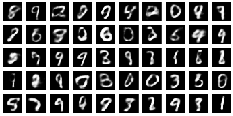
(1) random하게 noise vector 생성 뒤 visualize
def sample_vae(dec, n_samples=50):
    with torch.no_grad():
        ############# 순서 ####################
        # (1) sampling하기
        # (2) Sigmoid( Decoder ( sampling ) )
        # (3) Sigmoid의 결과값을 28x28로 reshape
        #######################################
        samples = torch.sigmoid(dec(torch.randn(n_samples, d).to(device)))
        samples = samples.view(n_samples, 28, 28).cpu().numpy()
    return samples
def plot_samples(samples, h=5, w=10):
    fig, axes = plt.subplots(nrows=h,
                             ncols=w,
                             figsize=(int(1.4 * w), int(1.4 * h)),
                             subplot_kw={'xticks': [], 'yticks': []})
    for i, ax in enumerate(axes.flatten()):
        ax.imshow(samples[i], cmap='gray')
plot_samples(sample_vae(Decoder))
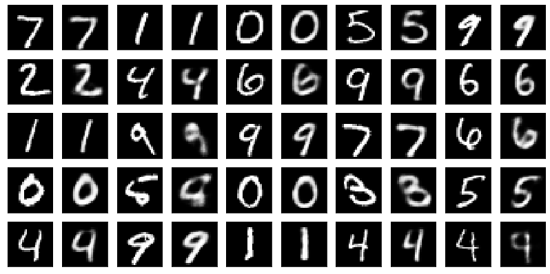
(2) test data에서 sampling하여 visualize
def plot_reconstructions(loss, model):
    with torch.no_grad():

        ## (1) test data의 첫 25개의 data를 샘플링
        batch = (test_loader.dataset.data[:25].float() / 255.)
        batch = batch.view(-1, D).to(device)

        ## (2) sampling한 것을 Decoder에 넣어서 output을 얻어냄
        _, rec = loss(batch, *model)

        ## (3) Sigmoid함수에 넣기
        rec = torch.sigmoid(rec)
        rec = rec.view(-1, 28, 28).cpu().numpy()
        batch = batch.view(-1, 28, 28).cpu().numpy()

        ## (4) Visualization
        fig, axes = plt.subplots(nrows=5, ncols=10, figsize=(14, 7),
                                 subplot_kw={'xticks': [], 'yticks': []})

        for i in range(25):
            axes[i % 5, 2 * (i // 5)].imshow(batch[i], cmap='gray')
            axes[i % 5, 2 * (i // 5) + 1].imshow(rec[i], cmap='gray')
plot_reconstructions(loss_fun, [Encoder, Decoder])