(PRML) Ch12.Continuous Latent Variables

( Skip the basic parts + not important contents )

12.Continuous Latent Variables

Ch 9) Probabilistic models with “DISCRETE” latent variables

Ch 12) Probabilistic models with “CONTINUOUS” latent variables

12-1. PCA (Principal Component Analysis)

PCA : used in..

• dimension reduction
• lossy data compression
• feature extraction
• data vizualization

2 common definitions of PCA

• 1) orthogonal projection of data into lower dimension linear space ( = principal subspace )

• 2) linear projection that minimizes the average projection cost

  ( = mean squared distance between data points & their projections)

12-1-1. Maximum variance formulation

\(D\) : original dimension

\(M\) : reduced dimension

example with 1D reduction (\(M=1\)):

• \(u_1\) : \(D\) dim vector
• \[u_1^Tu_1=1.\]

projected data

• mean : \(\mathbf{u}_{1}^{\mathrm{T}} \overline{\mathbf{x}}\)
  • where \(\overline{\mathbf{x}}=\frac{1}{N} \sum_{n=1}^{N} \mathbf{x}_{n}\)
• variance : \(\frac{1}{N} \sum_{n=1}^{N}\left\{\mathbf{u}_{1}^{\mathrm{T}} \mathbf{x}_{n}-\mathbf{u}_{1}^{\mathrm{T}} \overline{\mathbf{x}}\right\}^{2}=\mathbf{u}_{1}^{\mathrm{T}} \mathbf{S} \mathbf{u}_{1}\)
  • where \(\mathbf{S}=\frac{1}{N} \sum_{n=1}^{N}\left(\mathbf{x}_{n}-\overline{\mathbf{x}}\right)\left(\mathbf{x}_{n}-\overline{\mathbf{x}}\right)^{\mathrm{T}}\)

maximize \(\mathbf{u}_{1}^{\mathrm{T}} \mathbf{S} \mathbf{u}_{1}\) ,w.r.t \(\mathbf{u}_{1}\)

• with constraint \(\mathbf{u}_{1}^{\mathrm{T}} \mathbf{u}_{1}=1\)

  ( use Lagrange multiplier )

• \(\mathbf{u}_{1}^{\mathrm{T}} \mathbf{S} \mathbf{u}_{1}+\lambda_{1}\left(1-\mathbf{u}_{1}^{\mathrm{T}} \mathbf{u}_{1}\right)\).

  \(\mathbf{S u}_{1}=\lambda_{1} \mathbf{u}_{1}\).

  \(\therefore \mathbf{u}_{1}^{\mathrm{T}} \mathbf{S} \mathbf{u}_{1}=\lambda_{1}\).

• Variance will be maximum, if we set \(u_1\) equal to the eigenvector, that has largest eigenvalue \(\lambda_1\)

Generalization to \(M\) dimension

• \(M\) eigenvectors \(\mathbf{u}_{1}, \ldots, \mathbf{u}_{M}\)

  \(M\) largest eigenvalues \(\lambda_{1}, \ldots, \lambda_{M}\)

• Summary : PCA involves…

  • 1) evaluating \(\bar{\mathbf{x}}\) and \(S\) ( covariance matrix )
  • 2) find \(M\) eigenvectors of \(S\), corresponding to the \(M\) largest eigenvalues

• Computational cost

  • full eigenvector decomposition : \(O(D^3)\)

  • if project our data onto \(M\) PCs :

    ( using efficient techniques, such as “power method” : \(O(MD^2)\) )

    ( can also use EM algorithm )

12-1-2. Minimum-error formulation

alternative formulation of PCA, based on “PROJECTION ERROR MINIMIZATION”

• introduce complete orthonormal set of \(D\)-dimensional basis vectors \(\{u_i\}\)

  ( where \(i=1, \ldots, D\) and \(\mathbf{u}_{i}^{\mathrm{T}} \mathbf{u}_{j}=\delta_{i j}\))

each data point can be represented with linear combination

• \(\mathbf{x}_{n}=\sum_{i=1}^{D} \alpha_{n i} \mathbf{u}_{i}\).

  \(\alpha_{n j}=\mathbf{x}_{n}^{\mathrm{T}} \mathbf{u}_{j},\) (by orthonormality property)

  \(\therefore\) \(\mathbf{x}_{n}=\sum_{i=1}^{D}\left(\mathbf{x}_{n}^{\mathrm{T}} \mathbf{u}_{i}\right) \mathbf{u}_{i}\).

wish to use representation in restricted number \(M < D\)

approximate each datapoint as below : \(\tilde{\mathbf{x}}_{n}=\sum_{i=1}^{M} z_{n i} \mathbf{u}_{i}+\sum_{i=M+1}^{D} b_{i} \mathbf{u}_{i}\).

• \(\left\{z_{n i}\right\}\) depend on the particular data point
• \(\left\{b_{i}\right\}\) are constants

Goal : minimize \(J=\frac{1}{N} \sum_{n=1}^{N}\left\|\mathbf{x}_{n}-\tilde{\mathbf{x}}_{n}\right\|^{2}\).

• (1) w.r.t \(z_{ni}\) : \(z_{n j}=\mathbf{x}_{n}^{\mathrm{T}} \mathbf{u}_{j}\), where \(j=1, \ldots, M\)

• (2) w.r.t \(b_i\) : \(b_{j}=\overline{\mathbf{x}}^{\mathrm{T}} \mathbf{u}_{j}\) , where \(j=M+1, \ldots, D\)

\(\rightarrow\) substitute using (1), (2),

then \(\mathbf{x}_{n}-\tilde{\mathbf{x}}_{n}=\sum_{i=M+1}^{D}\left\{\left(\mathbf{x}_{n}-\overline{\mathbf{x}}\right)^{\mathrm{T}} \mathbf{u}_{i}\right\} \mathbf{u}_{i}\)

Thus, \(J=\frac{1}{N} \sum_{n=1}^{N}\left\|\mathbf{x}_{n}-\tilde{\mathbf{x}}_{n}\right\|^{2}=\frac{1}{N} \sum_{n=1}^{N} \sum_{i=M+1}^{D}\left(\mathbf{x}_{n}^{\mathrm{T}} \mathbf{u}_{i}-\overline{\mathbf{x}}^{\mathrm{T}} \mathbf{u}_{i}\right)^{2}=\sum_{i=M+1}^{D} \mathbf{u}_{i}^{\mathrm{T}} \mathbf{S} \mathbf{u}_{i}\)

Example with \(D=2\) and \(M=1\)

• minimize \(J=\mathbf{u}_{2}^{\mathrm{T}} \mathrm{Su}_{2},\)

  subject to \(\mathrm{u}_{2}^{\mathrm{T}} \mathbf{u}_{2}=1\)

• Loss function : \(\tilde{J}=\mathbf{u}_{2}^{\mathrm{T}} \mathbf{S} \mathbf{u}_{2}+\lambda_{2}\left(1-\mathbf{u}_{2}^{\mathrm{T}} \mathbf{u}_{2}\right)\)

  \(\rightarrow\) \(\mathbf{S u}_{2}=\lambda_{2} \mathbf{u}_{2}\)

• Summary

  minimizing average squared projection distance = maximum variance

general solution to minimizing \(J\) : \(\mathbf{S u}_{i}=\lambda_{i} \mathbf{u}_{i}\)

distortion measure : \(J=\sum_{i=M+1}^{D} \lambda_{i}\)

• ( = select e.v that those having \(D-M\) smallest eigenvalues )

• ( = choosing principal subspace, corresponding to \(M\) largest eigenvalues)

12-1-3. Applications of PCA

(1) PCA for data compression

PCA approximation to \(\tilde{x_n}\):

\(\begin{aligned} \tilde{\mathbf{x}}_{n} &=\sum_{i=1}^{M}\left(\mathbf{x}_{n}^{\mathrm{T}} \mathbf{u}_{i}\right) \mathbf{u}_{i}+\sum_{i=M+1}^{D}\left(\overline{\mathbf{x}}^{\mathrm{T}} \mathbf{u}_{i}\right) \mathbf{u}_{i} \\ &=\overline{\mathbf{x}}+\sum_{i=1}^{M}\left(\mathbf{x}_{n}^{\mathrm{T}} \mathbf{u}_{i}-\overline{\mathbf{x}}^{\mathrm{T}} \mathbf{u}_{i}\right) \mathbf{u}_{i} \end{aligned}\).

for each datapoint, we have replaced

• before) \(D\) dimension vector \(x_n\)
• after) \(M\) dimension vector with components \(\left(\mathbf{x}_{n}^{\mathrm{T}} \mathbf{u}_{i}-\overline{\mathbf{x}}^{\mathrm{T}} \mathbf{u}_{i}\right)\)

(2) PCA for data pre-processing

• dimension reduction (X)

  standardize (O)

Covariance matrix for standardized data :

• \(\rho_{i j}=\frac{1}{N} \sum_{n=1}^{N} \frac{\left(x_{n i}-\bar{x}_{i}\right)}{\sigma_{i}} \frac{\left(x_{n j}-\bar{x}_{j}\right)}{\sigma_{j}}\).

By using PCA, we can make more substantial normalization,

so that “different variables become decorrelated”

(1) write \(\mathbf{S u}_{i}=\lambda_{i} \mathbf{u}_{i}\) in the form \(\mathbf{S}\mathbf{U}=\mathbf{U}\mathbf{L}\)

• \(\mathbf{L}\) : \(D \times D\) diagonal matrix, with elements \(\lambda_i\)
• \(\mathbf{U}\) : \(D \times D\) orthogonal matrix, with columns \(\mathbf{u}_i\)

(2) transformed value \(\mathbf{y_n}\) : \(\mathbf{y}_{n}=\mathbf{L}^{-1 / 2} \mathbf{U}^{\mathrm{T}}\left(\mathbf{x}_{n}-\overline{\mathbf{x}}\right)\)

(3) \(\mathbf{y}_{n}=\mathbf{L}^{-1 / 2} \mathbf{U}^{\mathrm{T}}\left(\mathbf{x}_{n}-\overline{\mathbf{x}}\right)\)’s mean and variance

• mean : 0

• variance : \(I\) (identity matrix)

  \(\begin{aligned} \frac{1}{N} \sum_{n=1}^{N} \mathbf{y}_{n} \mathbf{y}_{n}^{\mathrm{T}} &=\frac{1}{N} \sum_{n=1}^{N} \mathbf{L}^{-1 / 2} \mathbf{U}^{\mathrm{T}}\left(\mathbf{x}_{n}-\overline{\mathbf{x}}\right)\left(\mathbf{x}_{n}-\overline{\mathbf{x}}\right)^{\mathrm{T}} \mathbf{U} \mathbf{L}^{-1 / 2} \\ &=\mathbf{L}^{-1 / 2} \mathbf{U}^{\mathrm{T}} \mathbf{S} \mathbf{U} \mathbf{L}^{-1 / 2}=\mathbf{L}^{-1 / 2} \mathbf{L} \mathbf{L}^{-1 / 2}=\mathbf{I} \end{aligned}\).

12-1-4. PCA for high-dimensional data

case of \(N<<D\)

\(\rightarrow\) computationally infeasible ( = \(O(D^3)\) )

How to solve?

(1) let \(\mathbf{X}\) to be \(N \times D\) dim, centered matrix

• \(n^{\text{th}}\) row : \(\left(\mathbf{x}_{n}-\overline{\mathbf{x}}\right)^{\mathrm{T}}\)

(2) Then, \(\mathbf{S}=\frac{1}{N} \sum_{n=1}^{N}\left(\mathbf{x}_{n}-\overline{\mathbf{x}}\right)\left(\mathbf{x}_{n}-\overline{\mathbf{x}}\right)^{\mathrm{T}}\) can be written as

• \(\mathbf{S}=N^{-1} \mathbf{X}^{\mathrm{T}} \mathbf{X}\).

(3) eigenvector equation

• \(\frac{1}{N} \mathbf{X}^{\mathrm{T}} \mathbf{X} \mathbf{u}_{i}=\lambda_{i} \mathbf{u}_{i}\).

• \(\frac{1}{N} \mathbf{X} \mathbf{X}^{\mathrm{T}}\left(\mathbf{X} \mathbf{u}_{i}\right)=\lambda_{i}\left(\mathbf{X} \mathbf{u}_{i}\right)\)…. ( pre-multiply both sides by \(\mathbf{X}\) )

• \(\frac{1}{N} \mathbf{X} \mathbf{X}^{\mathrm{T}} \mathbf{v}_{i}=\lambda_{i} \mathbf{v}_{i}\) …. ( define \(\mathbf{v}_{i}=\mathbf{X} \mathbf{u}_{i}\) )

  \(\rightarrow\) eigenvector equation for \(N \times N\) matrix \(N^{-1} XX^T\)

• \(\left(\frac{1}{N} \mathbf{X}^{\mathrm{T}} \mathbf{X}\right)\left(\mathbf{X}^{\mathrm{T}} \mathbf{v}_{i}\right)=\lambda_{i}\left(\mathbf{X}^{\mathrm{T}} \mathbf{v}_{i}\right)\).

  • \(\left(\mathbf{X}^{\mathrm{T}} \mathbf{v}_{i}\right)\) is an eigenvector of \(\mathbf{S}\) with eigenvalue \(\lambda_{i}\)

• \(\mathbf{u}_{i}=\frac{1}{\left(N \lambda_{i}\right)^{1 / 2}} \mathbf{X}^{\mathrm{T}} \mathbf{v}_{i}\\\) (after normalization)

(4) Summary

• from \(O(D^3)\) to \(O(N^3)\)

• first, evaluate \(XX^T\)

  then, find its eigenvectors & eigenvalues

  then, compute eigenvectors in the original data space, using \(\mathbf{u}_{i}=\frac{1}{\left(N \lambda_{i}\right)^{1 / 2}} \mathbf{X}^{\mathrm{T}} \mathbf{v}_{i}\\\)

12-2. Probabilsitic PCA (PPCA)

advantages compared with conventional PCA

• constrained form of the Gaussian distribution

• derive EM for PCA \(\rightarrow\) computationally efficient

• deal with missing values

• mixtures of PPCA can be formulated

• PPCA form the basis for Bayesian treatment of PCA

  ( = dimensionality of the principal subspace can be found automatically from the data )

• can be run generatively

  ( = sampling from the distribution )

Introduction

• Closely related to “factor analysis”
• example of linear-Gaussian framework
• formulation
  • explicit latent variable \(z\) ( = principal component )
  • define Gaussian prior over \(z\) ( = \(p(\mathbf{z})=\mathcal{N}(\mathbf{z} \mid \mathbf{0}, \mathbf{I})\) )
  • then, \(p(\mathbf{x} \mid \mathbf{z})=\mathcal{N}\left(\mathbf{x} \mid \mathbf{W} \mathbf{z}+\boldsymbol{\mu}, \sigma^{2} \mathbf{I}\right)\)

\(p(\mathbf{x} \mid \mathbf{z})=\mathcal{N}\left(\mathbf{x} \mid \mathbf{W} \mathbf{z}+\boldsymbol{\mu}, \sigma^{2} \mathbf{I}\right)\).

• mean : linear function of \(\mathbf{z}\)
  • ( \(W\) : \(D \times M\) matrix )
  • ( \(\mu\) : \(D\) dimensional vector )

Generative viewpoint

\(\mathbf{x}=\mathbf{W}\mathbf{z}+\boldsymbol{\mu}+\boldsymbol{\epsilon}\).

• \(z\) : \(M\) dim Gaussian latent variable
• \(\epsilon\) : \(D\) -dim noise variable, with covariance \(\sigma^2 I\)

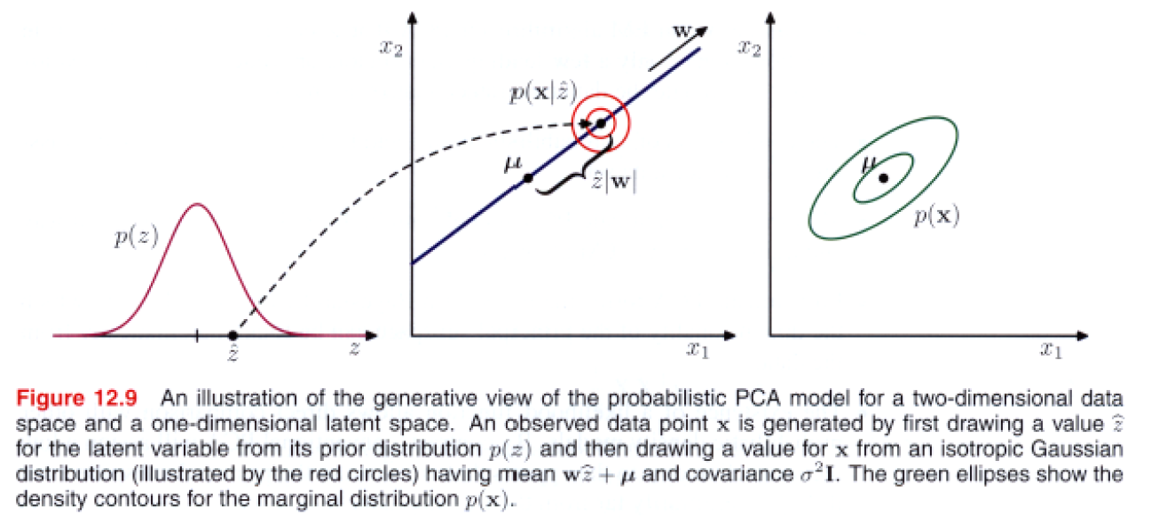
Marginal distribution ( predictive distribution ) \(p(x)\)

How to find parameters \(\mathbf{W}, \boldsymbol{\mu}\) and \(\sigma^{2}\) ?

\(\rightarrow\) likelihood function! need marginal distribution \(p(x)\)

\(p(\mathbf{x})=\int p(\mathbf{x} \mid \mathbf{z}) p(\mathbf{z}) \mathrm{d} \mathbf{z}\).

\(p(\mathbf{x})=\mathcal{N}(\mathbf{x} \mid \boldsymbol{\mu}, \mathbf{C})\).

• where \(\mathbf{C}=\mathbf{W} \mathbf{W}^{\mathrm{T}}+\sigma^{2} \mathbf{I}\)

proof )

\(\begin{aligned} \mathbb{E}[\mathbf{x}] &=\mathbb{E}[\mathbf{W} \mathbf{z}+\boldsymbol{\mu}+\boldsymbol{\epsilon}]=\boldsymbol{\mu} \\ \operatorname{cov}[\mathbf{x}] &=\mathbb{E}\left[(\mathbf{W} \mathbf{z}+\boldsymbol{\epsilon})(\mathbf{W} \mathbf{z}+\boldsymbol{\epsilon})^{\mathrm{T}}\right] \\ &=\mathbb{E}\left[\mathbf{W} \mathbf{z} \mathbf{z}^{\mathrm{T}} \mathbf{W}^{\mathrm{T}}\right]+\mathbb{E}\left[\boldsymbol{\epsilon} \boldsymbol{\epsilon}^{\mathrm{T}}\right]=\mathbf{W} \mathbf{W}^{\mathrm{T}}+\sigma^{2} \mathbf{I} \end{aligned}\).

To evaluate \(p(\mathbf{x})\), we need to evaluate \(C^{-1}\)

• where \(\mathbf{C}=\mathbf{W} \mathbf{W}^{\mathrm{T}}+\sigma^{2} \mathbf{I}\)

• thus, need inversion of \(D \times D\) matrix

• can be reduced, using \(\left(\mathbf{A}+\mathbf{B} \mathbf{D}^{-1} \mathbf{C}\right)^{-1}=\mathbf{A}^{-1}-\mathbf{A}^{-1} \mathbf{B}\left(\mathbf{D}+\mathbf{C A}^{-1} \mathbf{B}\right)^{-1} \mathbf{C A}^{-1}\)

  \(\rightarrow\) \(\mathrm{C}^{-1}=\sigma^{-1} \mathrm{I}-\sigma^{-2} \mathrm{WM}^{-1} \mathrm{~W}^{\mathrm{T}}\).

  where \(\mathbf{M}=\mathbf{W}^{T} \mathbf{W}+\sigma^{2} \mathbf{I}\)

• Thus, \(O(D^3)\) \(\rightarrow\) \(O(M^3)\)

Posterior distribution \(p(z\mid x)\)

\(p(\mathbf{z} \mid \mathbf{x})=\mathcal{N}\left(\mathbf{z} \mid \mathbf{M}^{-1} \mathbf{W}^{\mathrm{T}}(\mathbf{x}-\boldsymbol{\mu}), \sigma^{-2} \mathbf{M}\right)\).

• mean : depends on \(x\)
• cov : independent of \(x\)

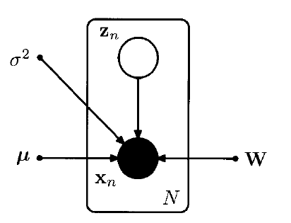
12-2-1. Maximum Likelihood PCA

expressed as a directed graph!

\(\begin{array}{l} \ln p\left(\mathbf{X} \mid \boldsymbol{\mu}, \mathbf{W}, \sigma^{2}\right)&=\sum_{n=1}^{N} \ln p\left(\mathbf{x}_{n} \mid \mathbf{W}, \boldsymbol{\mu}, \sigma^{2}\right) \\ &= -\frac{N D}{2} \ln (2 \pi)-\frac{N}{2} \ln |\mathbf{C}|-\frac{1}{2} \sum_{n=1}^{N}\left(\mathbf{x}_{n}-\boldsymbol{\mu}\right)^{\mathrm{T}} \mathbf{C}^{-1}\left(\mathbf{x}_{n}-\boldsymbol{\mu}\right) \end{array}\).

• if we solve MLE : \(\mu=\overline{\mathrm{x}}\).

  \(\ln p\left(\mathbf{X} \mid \mathbf{W}, \boldsymbol{\mu}, \sigma^{2}\right)=-\frac{N}{2}\left\{D \ln (2 \pi)+\ln \mid \mathbf{C}\mid+\operatorname{Tr}\left(\mathbf{C}^{-1} \mathbf{S}\right)\right\}\).

  • \(\mathbf{S}=\frac{1}{N} \sum_{n=1}^{N}\left(\mathbf{x}_{n}-\overline{\mathbf{x}}\right)\left(\mathbf{x}_{n}-\overline{\mathbf{x}}\right)^{\mathrm{T}}\).

Maximization of \(\ln p\left(\mathbf{X} \mid \boldsymbol{\mu}, \mathbf{W}, \sigma^{2}\right)\)

• \(\mathbf{W}_{\mathrm{ML}}=\mathbf{U}_{M}\left(\mathbf{L}_{M}-\sigma^{2} \mathbf{I}\right)^{1 / 2} \mathbf{R}\).
  • \(\mathbf{U}_{M}\) : \(D \times M\) matrix, of subset of the eigenvectors of the cov matrix \(S\)
  • \(\mathbf{L}_m\) : \(M \times M\) diagonal matrix ( with eigenvalues \(\lambda_i\) )
  • \(\mathbf{R}\) : arbitrary \(M \times M\) orthogonal matrix
• \(\sigma_{\mathrm{ML}}^{2}=\frac{1}{D-M} \sum_{i=M+1}^{D} \lambda_{i}\).

12-2-2. EM algorithm for PCA

PPCA : marginalization over a continuous latent variable \(z\)

( each data point \(x_n\) has its corresponding \(z_n\))

use EM algorithm to find MLE of parameters!

• adv 1) seems awkward.. but in HIGH DIMENSIONAL CASE : computational advantages!
• adv 2) can be extended to factor analysis
• adv 3) allows missing data to be handled

Complete-data log likelihood

\(\ln p\left(\mathbf{X}, \mathbf{Z} \mid \boldsymbol{\mu}, \mathbf{W}, \sigma^{2}\right)=\sum_{n=1}^{N}\left\{\ln p\left(\mathbf{x}_{n} \mid \mathbf{z}_{n}\right)+\ln p\left(\mathbf{z}_{n}\right)\right\}\).

\(\begin{aligned} \mathbb{E}[\ln p&\left.\left(\mathbf{X}, \mathbf{Z} \mid \boldsymbol{\mu}, \mathbf{W}, \sigma^{2}\right)\right]=-\sum_{n=1}^{N}\left\{\frac{D}{2} \ln \left(2 \pi \sigma^{2}\right)+\frac{1}{2} \operatorname{Tr}\left(\mathbb{E}\left[\mathbf{z}_{n} \mathbf{z}_{n}^{\mathrm{T}}\right]\right)\right.\\ &+\frac{1}{2 \sigma^{2}}\left\|\mathbf{x}_{n}-\boldsymbol{\mu}\right\|^{2}-\frac{1}{\sigma^{2}} \mathbb{E}\left[\mathbf{z}_{n}\right]^{\mathrm{T}} \mathbf{W}^{\mathrm{T}}\left(\mathbf{x}_{n}-\boldsymbol{\mu}\right) \\ &\left.+\frac{1}{2 \sigma^{2}} \operatorname{Tr}\left(\mathbb{E}\left[\mathbf{z}_{n} \mathbf{z}_{n}^{\mathrm{T}}\right] \mathbf{W}^{\mathrm{T}} \mathbf{W}\right)\right\} \end{aligned}\).

E-step

use old parameter values to evaluate

• \(\mathbb{E}\left[\mathbf{z}_{n}\right] =\mathbf{M}^{-1} \mathbf{W}^{\mathrm{T}}\left(\mathbf{x}_{n}-\overline{\mathbf{x}}\right)\).
• \(\mathbb{E}\left[\mathbf{z}_{n} \mathbf{z}_{n}^{\mathrm{T}}\right] =\sigma^{2} \mathbf{M}^{-1}+\mathbb{E}\left[\mathbf{z}_{n}\right] \mathbb{E}\left[\mathbf{z}_{n}\right]^{\mathrm{T}}\).

M-step

maximize w.r.t \(\mathbf{W}\) and \(\sigma^2\)

\[\begin{aligned} \mathbf{W}_{\text {new }}=&\left[\sum_{n=1}^{N}\left(\mathbf{x}_{n}-\overline{\mathbf{x}}\right) \mathbb{E}\left[\mathbf{z}_{n}\right]^{\mathrm{T}}\right]\left[\sum_{n=1}^{N} \mathbb{E}\left[\mathbf{z}_{n} \mathbf{z}_{n}^{\mathrm{T}}\right]\right]^{-1} \\ \sigma_{\text {new }}^{2}=& \frac{1}{N D} \sum_{n=1}^{N}\left\{\left\|\mathbf{x}_{n}-\overline{\mathbf{x}}\right\|^{2}-2 \mathbb{E}\left[\mathbf{z}_{n}\right]^{\mathrm{T}} \mathbf{W}_{\text {new }}^{\mathrm{T}}\left(\mathbf{x}_{n}-\overline{\mathbf{x}}\right)\right.\\ &\left.+\operatorname{Tr}\left(\mathbb{E}\left[\mathbf{z}_{n} \mathbf{z}_{n}^{\mathrm{T}}\right] \mathbf{W}_{\text {new }}^{\mathrm{T}} \mathbf{W}_{\text {new }}\right)\right\} \end{aligned}\]

Computational Efficiency

• eigen decomposition of
  • covariance matrix : \(O(D^3)\)
  • interested in \(M\) ev : \(O(MD^2)\)

• evaluation of covariance matrix : \(O(ND^2)\)

  ( \(N\) : number of data points )

• use “snapshot method”

  • eigenvectors are linear combinations of data vectors
  • avoid evaluation of covariance matrix
  • but \(O(N^3)\) ( not appropriate for large datasets )

• EM algorithm

  • do not construct covariance matrix explicitly

  • \(O(NDM)\).

    ( can be appropriate for large \(D\) and \(M<<D\) )

Others

• Deal with missing data

  ( by marginalizing over the distribution of unobserved)

• take limit \(\sigma^2 \rightarrow 0\), corresponding to standard PCA

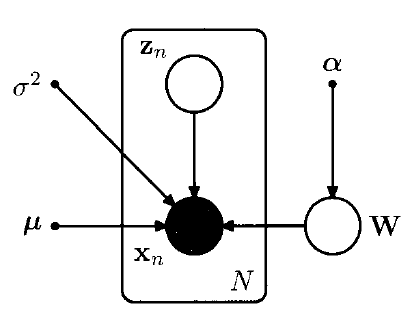
12-2-3. Bayesian PCA

Seek Bayesian approach to “model selection”

• Can be compared to different \(M\)

\(\rightarrow\) need to marginalize out \(\mu, \mathrm{W}, \text { and } \sigma^{2}\)

Evidence Approximation

• choice of prior over \(\mathbf{W}\)

  ( allows surplus dimensions in the principal subspace to be pruned out)

  \(\rightarrow\) ARD (Automatic Relevance Determination)

ARD (Automatic Relevance Determination)

• each Gaussian has independent variance, governed by hyperparameter \(\alpha_i\)
• \(p(\mathbf{W} \mid \boldsymbol{\alpha})=\prod_{i=1}^{M}\left(\frac{\alpha_{i}}{2 \pi}\right)^{D / 2} \exp \left\{-\frac{1}{2} \alpha_{i} \mathbf{w}_{i}^{\mathrm{T}} \mathbf{w}_{i}\right\}\).

• 

• \(\alpha_i \rightarrow \infty\) = \(w_i \rightarrow 0\)

• “effective dimensionality of the principal subspace is then determined by the number of finite \(\alpha_i\) values,

  and the corresponding vectors \(w_i\) can be thought of as ‘relevant’ for modeling the data distribution

Estimation of \(\alpha\)

• \(\alpha_i\) are re-estimated during training

• by maximizing the log marginal likelihood :

  \(p\left(\mathbf{X} \mid \boldsymbol{\alpha}, \boldsymbol{\mu}, \sigma^{2}\right)=\int p\left(\mathbf{X} \mid \mathbf{W}, \boldsymbol{\mu}, \sigma^{2}\right) p(\mathbf{W} \mid \boldsymbol{\alpha}) \mathrm{d} \mathbf{W}\).

• intractable! use Laplace approximation

• Result : \(\alpha_{i}^{\text {new }}=\frac{D}{\mathbf{w}_{i}^{\mathrm{T}} \mathbf{w}_{i}}\)

E-step

use old parameter values to evaluate

• \(\mathbb{E}\left[\mathbf{z}_{n}\right] =\mathbf{M}^{-1} \mathbf{W}^{\mathrm{T}}\left(\mathbf{x}_{n}-\overline{\mathbf{x}}\right)\).
• \(\mathbb{E}\left[\mathbf{z}_{n} \mathbf{z}_{n}^{\mathrm{T}}\right] =\sigma^{2} \mathbf{M}^{-1}+\mathbb{E}\left[\mathbf{z}_{n}\right] \mathbb{E}\left[\mathbf{z}_{n}\right]^{\mathrm{T}}\).

M-step

maximize w.r.t \(\mathbf{W}\) and \(\sigma^2\)

\(\begin{aligned} \mathbf{W}_{\text {new }}&=\left[\sum_{n=1}^{N}\left(\mathbf{x}_{n}-\overline{\mathbf{x}}\right) \mathbb{E}\left[\mathbf{z}_{n}\right]^{\mathrm{T}}\right]\left[\sum_{n=1}^{N} \mathbb{E}\left[\mathbf{z}_{n} \mathbf{z}_{n}^{\mathrm{T}}\right]+\sigma^{2} \mathbf{A}\right]^{-1} \\ \sigma_{\text {new }}^{2}=& \frac{1}{N D} \sum_{n=1}^{N}\left\{\left\|\mathbf{x}_{n}-\overline{\mathbf{x}}\right\|^{2}-2 \mathbb{E}\left[\mathbf{z}_{n}\right]^{\mathrm{T}} \mathbf{W}_{\text {new }}^{\mathrm{T}}\left(\mathbf{x}_{n}-\overline{\mathbf{x}}\right)\right.\\ &\left.+\operatorname{Tr}\left(\mathbb{E}\left[\mathbf{z}_{n} \mathbf{z}_{n}^{\mathrm{T}}\right] \mathbf{W}_{\text {new }}^{\mathrm{T}} \mathbf{W}_{\text {new }}\right)\right\} \end{aligned}\).

where \(\mathbf{A}=\operatorname{diag}\left(\alpha_{i}\right) .\)

12-2-4. Factor Analysis

• linear-Gaussian latent variable model

• closely related to PPCA

  ( difference ) conditional distribution : diagonal covariance

  \(p(\mathbf{x} \mid \mathbf{z})=\mathcal{N}(\mathbf{x} \mid \mathbf{W} \mathbf{z}+\boldsymbol{\mu}, \boldsymbol{\Psi})\).

  • where \(\Psi\) is a \(D \times D\) diagonal matrix

“factor loadings”

• Columns of \(\mathbf{W}\)

• capture the correlation between observation variables

“uniqueness”

• diagonal elements of \(\mathbf{\Psi}\)
• represent the independent noise variance

Marginal distribution for the observed variable

\(p(\mathbf{x})=\mathcal{N}(\mathbf{x} \mid \boldsymbol{\mu}, \mathbf{C})\).

• where \(\mathbf{C}=\mathbf{W} \mathbf{W}^{\mathrm{T}}+\boldsymbol{\Psi}\)

  ( PPCA : \(\mathbf{C}=\mathbf{W} \mathbf{W}^{\mathrm{T}}+\sigma^{2} \mathbf{I}\) )

• like PPCA, model is invariant to the rotations in the latent space

Unlike PPCA, there is no longer closed form!

\(\rightarrow\) use EM algorithm

E-step

\(\begin{aligned} \mathbb{E}\left[\mathbf{z}_{n}\right] &=\mathbf{G} \mathbf{W}^{\mathrm{T}} \boldsymbol{\Psi}^{-1}\left(\mathbf{x}_{n}-\overline{\mathbf{x}}\right) \\ \mathbb{E}\left[\mathbf{z}_{n} \mathbf{z}_{n}^{\mathrm{T}}\right] &=\mathbf{G}+\mathbb{E}\left[\mathbf{z}_{n}\right] \mathbb{E}\left[\mathbf{z}_{n}\right]^{\mathrm{T}} \end{aligned}\).

where \(\mathbf{G}=\left(\mathbf{I}+\mathbf{W}^{\mathrm{T}} \boldsymbol{\Psi}^{-1} \mathbf{W}\right)^{-1}\).

• need inversion of \(M \times M\) matrices ( not \(D \times D\))

M-step

\(\begin{aligned} \mathbf{W}^{\text {new }} &=\left[\sum_{n=1}^{N}\left(\mathbf{x}_{n}-\overline{\mathbf{x}}\right) \mathbb{E}\left[\mathbf{z}_{n}\right]^{\mathrm{T}}\right]\left[\sum_{n=1}^{N} \mathbb{E}\left[\mathbf{z}_{n} \mathbf{z}_{n}^{\mathrm{T}}\right]\right]^{-1} \\ \boldsymbol{\Psi}^{\text {new }} &=\operatorname{diag}\left\{\mathbf{S}-\mathbf{W}_{\text {new }} \frac{1}{N} \sum_{n=1}^{N} \mathbb{E}\left[\mathbf{z}_{n}\right]\left(\mathbf{x}_{n}-\overline{\mathbf{x}}\right)^{\mathrm{T}}\right\} \end{aligned}\)/

12-3. Kernel PCA

replacing the scalar products with NON-linear kernel

Review

• PCs are defined by eigenvectors \(u_i\) of covariance matrix \(S\)
• \(\mathbf{S u}_{i}=\lambda_{i} \mathbf{u}_{i}\).
  • \(\mathbf{S}=\frac{1}{N} \sum_{n=1}^{N} \mathbf{x}_{n} \mathbf{x}_{n}^{\mathrm{T}}\) : \(D \times D\) sample covariance matrix
  • \(\mathbf{u}_{i}^{\mathrm{T}} \mathbf{u}_{i}=1\) : normalized eigenvector

Nonlinear transformation \(\phi(x)\)

• perform standard PCA in the “feature space”

  ( = “nonlinear” PC model in the “original model”)

• \(\mathrm{Cv}_{i}=\lambda_{i} \mathbf{v}_{i}\).

  • \(\mathbf{C}=\frac{1}{N} \sum_{n=1}^{N} \phi\left(\mathbf{x}_{n}\right) \phi\left(\mathbf{x}_{n}\right)^{\mathrm{T}}\) : \(M \times M\) sample covariance matrix
  • \(\lambda_{i} \mathbf{v}_{i}= \frac{1}{N} \sum_{n=1}^{N} \phi\left(\mathbf{x}_{n}\right)\left\{\phi\left(\mathbf{x}_{n}\right)^{\mathrm{T}} \mathbf{v}_{i}\right\}\).
    • \(\mathbf{v}_{i}=\sum_{n=1}^{N} a_{i n} \phi\left(\mathbf{x}_{n}\right)\).

[ Eigenvector equation ]

\(\mathrm{Cv}_{i}=\lambda_{i} \mathbf{v}_{i}\).

\(\frac{1}{N} \sum_{n=1}^{N} \phi\left(\mathbf{x}_{n}\right) \phi\left(\mathbf{x}_{n}\right)^{\mathrm{T}} \sum_{m=1}^{N} a_{i m} \phi\left(\mathbf{x}_{m}\right)=\lambda_{i} \sum_{n=1}^{N} a_{i n} \phi\left(\mathbf{x}_{n}\right)\).

( since \(k\left(\mathbf{x}_{n}, \mathbf{x}_{m}\right)=\phi\left(\mathbf{x}_{n}\right)^{\mathrm{T}} \phi\left(\mathrm{x}_{m}\right)\) )

\(\frac{1}{N} \sum_{n=1}^{N} k\left(\mathbf{x}_{l}, \mathbf{x}_{n}\right) \sum_{m=1}^{m} a_{i m} k\left(\mathbf{x}_{n}, \mathbf{x}_{m}\right)=\lambda_{i} \sum_{n=1}^{N} a_{i n} k\left(\mathbf{x}_{l}, \mathbf{x}_{n}\right)\).

( as matrix notation )

\(\mathbf{K}^{2} \mathbf{a}_{i}=\lambda_{i} N \mathbf{K} \mathbf{a}_{i}\).

\(\mathbf{K} \mathbf{a}_{i}=\lambda_{i} N \mathbf{a}_{i}\).

Normalization condition is obtained!

• proof )

  \(1=\mathbf{v}_{i}^{\mathrm{T}} \mathbf{v}_{i}=\sum_{n=1}^{N} \sum_{m=1}^{N} a_{i n} a_{i m} \phi\left(\mathbf{x}_{n}\right)^{\mathrm{T}} \boldsymbol{\phi}\left(\mathbf{x}_{m}\right)=\mathbf{a}_{i}^{\mathrm{T}} \mathbf{K} \mathbf{a}_{i}=\lambda_{i} N \mathbf{a}_{i}^{\mathrm{T}} \mathbf{a}_{i}\).

Projection of point \(\mathbf{x}\) onto eigenvector \(i\):

• \(y_{i}(\mathbf{x})=\boldsymbol{\phi}(\mathbf{x})^{\mathrm{T}} \mathbf{v}_{i}=\sum_{n=1}^{N} a_{i n} \boldsymbol{\phi}(\mathbf{x})^{\mathrm{T}} \boldsymbol{\phi}\left(\mathbf{x}_{n}\right)=\sum_{n=1}^{N} a_{i n} k\left(\mathbf{x}, \mathbf{x}_{n}\right)\).

Original PCA vs Kernel PCA

• original) can have at most \(D\) PCs

• kernel) can exceed \(D\) PCs

  ( but cannot exceed \(N\), which is the number of data points, since covariance matrix in feature space has rank at most equal to \(N\) )

Centralize

• cannot simply compute and then subtract off the mean

• should be done “in terms of the kernel function”

  \(\widetilde{\phi}\left(\mathbf{x}_{n}\right)=\phi\left(\mathbf{x}_{n}\right)-\frac{1}{N} \sum_{l=1}^{N} \phi\left(\mathbf{x}_{l}\right)\).

Gram matrix : \(\widetilde{\mathbf{K}}=\mathbf{K}-\mathbf{1}_{N} \mathbf{K}-\mathbf{K} \mathbf{1}_{N}+\mathbf{1}_{N} \mathbf{K} \mathbf{1}_{N}\)

Example )

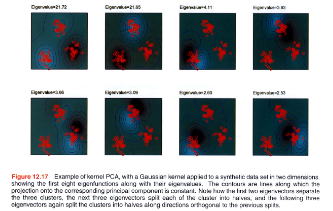
• Gaussian’ kernel : \(k\left(\mathbf{x}, \mathbf{x}^{\prime}\right)=\exp \left(-\left\|\mathbf{x}-\mathbf{x}^{\prime}\right\|^{2} / 0.1\right)\)

• lines correspond to contours,

  \(\phi(\mathbf{x})^{\mathrm{T}} \mathbf{v}_{i}=\sum^{N} a_{i n} k\left(\mathbf{x}, \mathbf{x}_{n}\right)\).

Disadvantage of Kernel PCA

• involves finding eigenvector of \(N \times N\) matrix \(\tilde{\mathbf{K}}\) ( not \(D \times D\) matrix \(S\) )

  \(\rightarrow\) for large datasets, approximation is needed

• standard PCA ) we can approximate a data vector \(x_n\) by \(\hat{x_n}\)

  like \(\widehat{\mathbf{x}}_{n}=\sum_{i=1}^{L}\left(\mathbf{x}_{n}^{\mathrm{T}} \mathbf{u}_{i}\right) \mathbf{u}_{i}\).

  kernel PCA) not possible

12-4. Nonlinear Latent Variable Models

generalization of this framework to “nonlinear” or “non-Gaussian”

12-4-1. ICA (Independent Component Analysis)

Framework

• observed variables are related linearly to the latent variables

• latent distribution is “NON-GAUSSIAN”

  \(p(\mathbf{z})=\prod_{j=1}^{M} p\left(z_{j}\right)\).

12-4-2. Autoassociative Neural Networks

NN has been used for dimensionality reduction

minimize some measure of the reconstruction error

• \(E(\mathbf{w})=\frac{1}{2} \sum_{n=1}^{N}\left\|\mathbf{y}\left(\mathbf{x}_{n}, \mathbf{w}\right)-\mathbf{x}_{n}\right\|^{2}\).

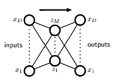
• two layers of weights
• equivalent to linear PCA

Limitations of a linear dimensionality could be overcome by NON-LINEAR activation functions

( additional hidden layers are permitted ! )

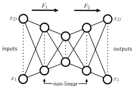
• four layer
• sigmoidal nonlinear activation
• not being limited to linear transformations!
• nonlinear optimization problem