Are Transformers Effective for Time Series Forecasting?

Abstract
Introduction
Preliminaries
Transformoer-Based LTSF Solutions
Embarassingly Simple Baseline
Experiments
Implementation Details
LTSF & STSF
Distribution Shift

0. Abstract

surge of Transformer-based solutions for the long-term time series forecasting (LTSF) task

\(\rightarrow\) this paper : question the validity of this line of research

Transformers : most successful solution to extract the semantic correlations among the elements in a long sequence.

However, in time series modeling, we are to extract the temporal relations in an ordered set of continuous points

[ Transformer ] positional encoding & tokens to embed sub-series

facilitate preserving some ordering information….

\(\rightarrow\) BUT the nature of the permutation-invariant self-attention mechanism inevitably results in temporal information loss

\(\rightarrow\) introduce a set of embarrassingly simple one-layer linear models named LTSF-Linear

https://github.com/cure-lab/LTSFLinear.

1. Introduction

The main working power of Transformers: multi-head self-attention mechanism

\(\rightarrow\) capability of extracting semantic correlations among elements in a long sequence

Problems of self-attention in TS :

permutation invariant & “anti-order” to some extent

using various types of positional encoding…? still inevitable to have temporal information loss

( NLP : not a serious concern for semantic rich applications )

( TS : usually a lack of semantics in the numerical data itself )

\(\rightarrow\) order itself plays the most crucial role

Q. Are Transformers really effective for long-term time series forecasting?

(non-Transformer) Baselines ( used in Transformer-based papers )

perform autoregressive or iterated multi-step (IMS) forecasting
- suffer from significant error accumulation effects for the LTSF problem

\(\rightarrow\) We challenge Transformer-based LTSF solutions with direct multi-step (DMS) forecasting strategies to validate their real performance

Hypothesize that long-term forecasting is only feasible for those time series with a relatively clear trend and periodicity.

\(\rightarrow\) linear models can already extract such information!

\(\rightarrow\) introduce a set of embarrassingly simple model, LTSF-Linear

LTSF-Linear

regresses historical time series with a one-layer linear model to forecast future time series directly.
conduct extensive experiments on nine widely-used benchmark datasets
show that LTSF-Linear outperforms existing complex Transformerbased models in all cases, and often by a large margin (20% ∼ 50%).
existing Transformers : most of them fail to extract temporal relations from long sequences
- the forecasting errors are not reduced (sometimes even increased) with the increase of look-back window sizes.
conduct various ablation studies on existing Transformer-based TSF solutions

2. Preliminaries: TSF Problem Formulation

Notation

number of variates : \(C\)
historical data : \(\mathcal{X}=\left\{X_1^t, \ldots, X_C^t\right\}_{t=1}^L\)
- lookback window size : \(L\)
- \(i_{t h}\) variate at the \(t_{t h}\) time step : \(X_i^t\)

TSF task: predict \(\hat{\mathcal{X}}=\left\{\hat{X}_1^t, \ldots, \hat{X}_C^t\right\}_{t=L+1}^{L+T}\)

iterated multi-step (IMS) forecasting : learns a single-step forecaster & iteratively applies it
direct multistep (DMS) forecasting : directly optimizes the multi-step forecasting objective

IMS vs DMS

IMS ) have smaller variance thanks to the autoregressive estimation procedure
DMS) less error accumulation effects.

\(\rightarrow\) IMS forecasting is preferable when ….

(1) highly-accurate single-step forecaster
(2) \(T\) is relatively small

\(\rightarrow\) DMS forecasting is preferable when ….

(1) hard to obtain an unbiased single-step forecasting model
(2) \(T\) is large.

3. Transformer-Based LTSF Solutions

Transformer-based models to LTSF problems?

Limitations

(1) quadratic time/memory complexity
(2) error accumulation by autoregressive decoder
- Informer : reduce complexity & DMS forecasting
- etc) xxformers…

(1) TS decomposition

Common in TSF : normalization with zero-mean

Autoformer : applies seasonal-trend decomposition behind each neural block

TREND : MA kernel on the input sequence to extract the TREND
SEASONALITY : original - TREND

FEDformer : ( on top of Autoformer )

proposes the mixture of experts’ strategies to mix the TREND components extracted by MA kernels with various kernel sizes.

(2) Input Embedding

self-attention layer : cannot preserve the positional information of the time series.

Local positional information ( i.e. the ordering of time series ) is important

Global temporal information ( such as hierarchical timestamps (week, month, year) and agnostic timestamps (holidays and events) ) is also informative

SOTA Transformer : inject several embeddings

fixed positional encoding
channel projection embedding
learnable temporal embeddings
temporal embeddings with a temporal convolution layer
learnable timestamps

(3) Self-attention

Vanilla Transformer : \(O\left(L^2\right)\) ( too large )

Recent works propose two strategies for efficiency

(1) LogTrans, Pyraformer
- explicitly introduce a sparsity bias into the self-attention scheme.
- ( LogTrans ) uses a Logsparse mask to reduce the computational complexity to \(O(\log L)\)
- ( Pyraformer ) adopts pyramidal attention that captures hierarchically multi-scale temporal dependencies with an \(O(L)\) time and memory complexity
(2) Informer, FEDformer, Autoformer
- use the low-rank property in the self-attention matrix.
- ( Informer ) proposes a ProbSparse self-attention mechanism and a self-attention distilling operation to decrease the complexity to \(O(L \log L)\),
- ( FEDformer ) designs a Fourier enhanced block and a wavelet enhanced block with random selection to obtain \(O(L)\) complexity.
(3) Autoformer
- designs a series-wise auto-correlation mechanism to replace the original self-attention layer.

(4) Decoders

Vanilla Transformer decoder

outputs sequences in an autoregressive manner
resulting in a slow inference speed and error accumulation effects

( especially for long-term predictions )

Use DMS strategies

Informer : designs a generative-style decoder for DMS forecasting.
Pyraformer : uses a FC layer concatenating Spatio-temporal axes as the decoder.
Autoformer : sums up two refined decomposed features from trend-cyclical components and the stacked auto-correlation mechanism for seasonal components to get the final prediction.
FEDformer : uses a decomposition scheme with the proposed frequency attention block to decode the final results.

The premise of Transformer models : semantic correlations between paired elements

self-attention mechanism itself is permutation-invariant

\(\rightarrow\) capability of modeling temporal relations largely depends on positional encodings
there are hardly any point-wise semantic correlations between them

TS modeling

mainly interested in the temporal relations among a continuous set of points

& order of these elements ( instead of the paired relationship ) plays the most crucial role
positional encoding and using tokens :
- not sufficient! TEMPORAL INFORMATION LOSS!

\(\rightarrow\) Revisit the effectiveness of Transformer-based LTSF solutions.

4. An Embarrassingly Simple Baseline

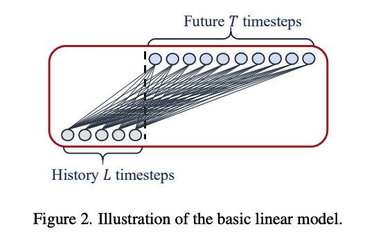
(1) Linear

LTSF-Linear: \(\hat{X}_i=W X_i\),

\(W \in \mathbb{R}^{T \times L}\) : linear layer along the temporal axis
\(\hat{X}_i\) and \(X_i\) : prediction and input for each \(i_{t h}\) variate

( LTSF-Linear shares weights across different variates & does not model any spatial correlations )

[Linear] Vanilla Linear : 1-layer Linear model

2 variantes :

[DLinear] = Linear + Decomposition
[NLinear] = Linear + Normalization

DLinear

( enhances the performance of a vanilla linear when there is a clear trend in the data. )

step 1) decomposes a raw data input into a TREND & REMAINDER
- use MA kernel
step 2) two 1-layer linear layer
- one for TREND
- one for REMAINDER
step 3) sum TREND & REMAINDER

NLinear

( when there is a distribution shift )

step 1) subtracts the input by the last value of the sequence
step 2) one 1-layer linear layer
step 3) add the subtracted value

5. Experiments

(1) Experimental Settings

a) Dataset

ETT (Electricity Transformer Temperature)

ETTh1, ETTh2, ETTm1, ETTm2

Traffic, Electricity, Weather, ILI, ExchangeRate

\(\rightarrow\) all of them are MTS

b) Compared Methods

5 transformer based methods

FEDformer, Autoformer, Informer, Pyraformer, LogTrans

naive DMS method:

Closest Repeat (Repeat)

( two variants of FEDformer )

compare with the better accuracy, FEDformer-f via Fourier Transform

(2) Comparison with Transformers

a) Quantitative results

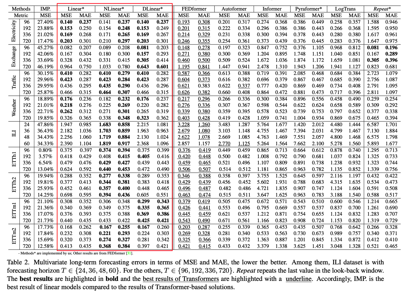
MTS forecasting

( note: LTSFLinear even does not model correlations among variates )

UTS forecasting (appendix)

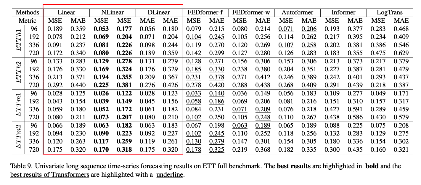
FEDformer

achieves competitive forecasting accuracy on ETTh1.
reason) FEDformer employs classical time series analysis techniques such as frequency processing
- which brings in TS inductive bias & benefits the ability of temporal feature extraction.

Summary

(1) existing complex Transformer-based LTSF solutions are not seemingly effective
(2) surprising result : naive Repeat outperforms all Transformer-based methods on Exchange-Rate

\(\rightarrow\) due to wrong prediction of trends in Transformer-based solutions
- overfit toward sudden change noises in the training data

b) Qualitative results

the prediction results on 3 TS datasets

input length \(L\) = 96
output length \(T\) = 336

[ Electricity and ETTh2 ] Transformers fail to capture the scale and bias of the future data

[ Exchange-Rate ] hardly predict a proper trend on aperiodic data

(3) More Analyses on LTSF-Transformers

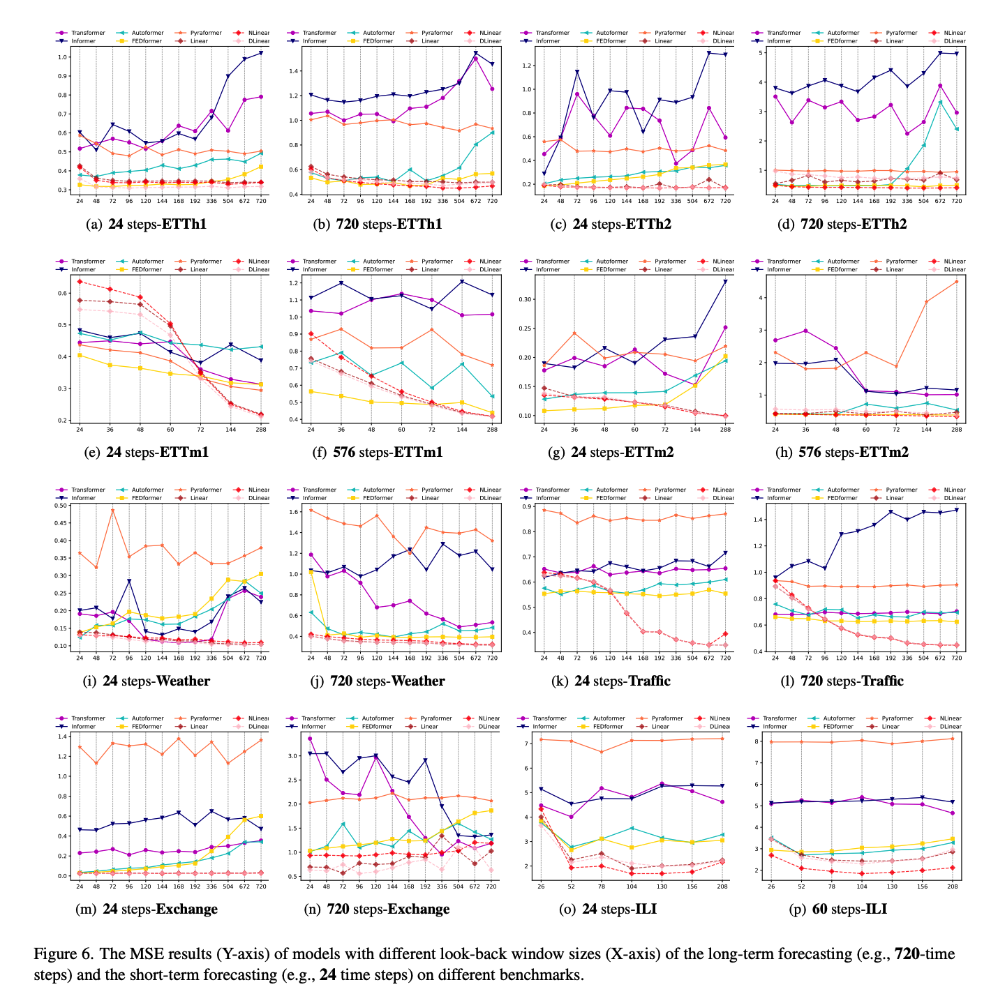
Q1. Can existing LTSF-Transformers extract temporal relations well from longer input sequences?

Size of the look-back window \(L\)

greatly impacts forecasting accuracy

Powerful TSF model with a strong temporal relation extraction capability :

larger \(L\), better results!

To study the impact of \(L\)…

conduct experiments with \(L \in\) \(\{24,48,72,96,120,144,168,192,336,504,672,720\}\)
where \(T\) = 720

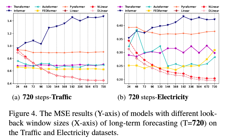
existing Transformer-based models’ performance deteriorates or stays stable, when larger \(L\)
( \(\leftrightarrow\) LTSF-Linear : boosted with larger \(L\) )

\(\rightarrow\) Transformers : tend to overfit temporal noises

( thus input size 96 is exactly suitable for most Transformers )

Q2. What can be learned for long-term forecasting?

Hypothesize that long-term forecasting depends on whether models can capture the trend and periodicity well only.

( That is, the farther the forecasting horizon, the less impact the look-back window itself has. )

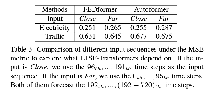
Experiment

\(T\) = 720 time steps
Lookback \(L\) = 96
- ver 1) original input \(\mathrm{L}=96\) setting (called Close)
- ver 2) far input \(\mathrm{L}=96\) setting (called Far)

…

6. Implementation Details

For existing Transformer-based TSF solutions:

Autoformer, Informer, and the vanilla Transformer : from Autoformer [28]
FEDformer and Pyraformer : from their respective code

( + adopt their default hyper-parameters to train the models )