(paper 69) Efficient Training of Visual Transformers with Small Datasets

Efficient Training of Visual Transformers with Small Datasets

Contents

1. Abstract
2. Introduction
   1. Advantage & Disadvantage of VTs
   2. Proposal
   3. Contribution
3. Preliminaries
4. Dense Relative Localization Task
5. Experiments
   1. Datasets
   2. From Scratch
   3. Fine Tuning

0. Abstract

Visual Transformers (VTs) : compared to CNN…

• 1) can capture GLOBAL relations between image elements

• 2) potentially have a LARGER representation

• BUT lack of the typical convolutional inductive bias

  \(\rightarrow\) need more data

(1) Empirically analyze different VTs

• show that their performance on smaller datasets can be largely different

(2) Propose an auxiliary SSL task

• extract additional information from images with only a negligible computational overhead

• used jointly with the standard (supervised) training

(code) https://github.com/yhlleo/VTs-Drloc.

1. Introduction

Visual Transformers (VTs)

• alternative to standard CNN ( inspired by Transformer )
• pioneering work : ViT
  • step 1) image is split using a grid of non-overlapping patches
  • step 2) each patch is linearly projected in the input embedding space ( = token )
  • step 3) all the tokens are processed by MHAs & FFNNs

(1) Advantage & Disadvantage of VTs

Advantage of VTs :

“use the attention layers to model GLOBAL relations between tokens”

( \(\leftrightarrow\) CNN : receptive field of the kernels locally limits the type of relations )

Disadvantage of VTs :

“increased representation capacity comes at a price”

• at the lack of the typical ”CNN inductive biases”
  • 1) locality
  • 2) translation invariance
  • 3) hierarchical structure ofvisual information

\(\rightarrow\) need a lot of data!

To alleviate this problem …. variants of VTs

• common idea : HYBRID ( = mix convolutional layers with attention layers )
  • to provide a local inductive bias to the VT.
  • enjoy the advantages of both paradigms :
    • ATTENTION ) model long-range dependencies
    • CONVOLUTION ) emphasize the local properties
• BUT still not clear what is the behaviour of these networks when trained on medium-small datasets.

(2) Proposal

(1) compare VTs… by either

• a) training from scratch
• b) fine-tuning

on medium-small datasets

\(\rightarrow\) Empirically show that classification accuracy with smaller datasets largely varies.

(2) Propose auxiliary SSL pretext task

• & corresponding loss function to regularize training in a small training set

Proposed task

• based on (unsupervised) learning the spatial relations between the output token embeddings

• densely sample random pairs from the final embedding grid

  & for each pair, guess the corresponding GEOMETRIC DISTANCE.

• network needs to encode both **1) local ** and **2) contextual ** information in each embedding

(3) Contribution

1. empirically compare different VTs
2. propose a RELATIVE LOCALIZATION auxiliary task for VT training regularization
3. show that this task is beneficial to speed-up training & improve generaization ability

2. Preliminaries

VT network

• [input] image split in a grid of K × K patches
• [process]
  • each patch is projected in the input embedding space
  • output : K × K input tokens
• [model] model ”pairwise relations” over the token intermediate representation

VT network with HYBRID architecture

( = second-generation VT )

usually reshape the sequence of these token embeddings in a spatial grid

• to enable convolutional operations

  ( by using convolutions/pooling ….. initial K × K token grid can be reduced )

• final embedding grid : k × k ( where k \(\leq\) K )

final k × k grid of embeddings

• representation of whole input image
• used for discriminative task
  • ex) include “class token” over the whole grid
  • ex) apply GAP

apply small MLP head!

• outputs a posterior distn over target classes

.

3. Dense Relative Localization Task

Goal of our regularization task :

• encourage the VT to learn ”spatial” information without using additional manual annotations

By densely sampling multiple embedding pairs for each image

& guess their relative distances

Notation

• input image : \(x\)
• \(k \times k\) grid of final embeddings : \(G_x=\left\{\mathbf{e}_{i, j}\right\}_{1 \leq i, j \leq k}\)
  • where \(\mathbf{e}_{i, j} \in \mathbb{R}^d\), and \(d\) is the dimension of the embedding space

Procedure

step 1)

For each \(G_x\) ……… randomly sample multiple ”pairs of embeddings”

step 2)

For each pair \(\left(\mathbf{e}_{i, j}, \mathbf{e}_{p, h}\right)\) …….. compute the 2D normalized target translation offset \(\left(t_u, t_v\right)^T\)

• $$t_u=\frac{

  i-p

  }{k}, \quad t_v=\frac{

  j-h

  }{k}, \quad\left(t_u, t_v\right)^T \in[0,1]^2$$.

step 3)

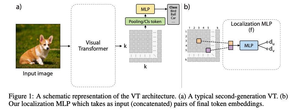
pair \(\left(\mathbf{e}_{i, j}, \mathbf{e}_{p, h}\right)\) are concatenated

& input to small MLP (Fig. 1 (b))

• predicts the relative distance between two positions on grid

Dense Relative Localization Loss :

$$\mathcal{L}{d r l o c}=\sum{x \in B} \mathbb{E}{\left(\mathbf{e}{i, j}, \mathbf{e}_{p, h}\right) \sim G_x}\left[\left

\left(t_u, t_v\right)^T-\left(d_u, d_v\right)^T\right

_1\right]$$.

• Let \(\left(d_u, d_v\right)^T=\) \(f\left(\mathbf{e}_{i, j}, \mathbf{e}_{p, h}\right)^T\).
• given a mini-batch \(B\) of \(n\) images

\(\mathcal{L}_{\text {drloc }}\) is added to the standard cross-entropy loss \(\left(\mathcal{L}_{c e}\right)\)

Final loss : \(\mathcal{L}_{t o t}=\mathcal{L}_{\text {ce }}+\lambda \mathcal{L}_{\text {drloc }}\)

• \(\lambda=0.1\) : in T2T and CvT
• \(\lambda=0.5\) : in Swin

4. Experiments

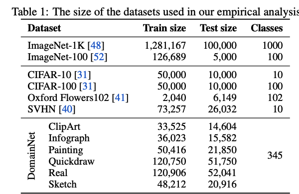
(1) Dataset

.

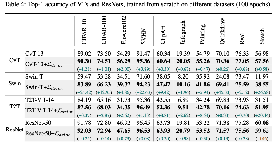
(2) From Scratch

.

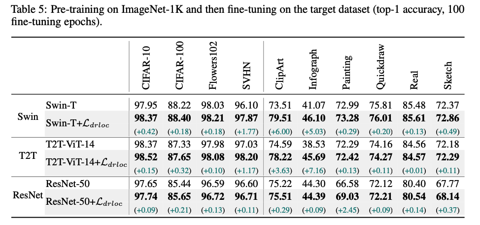
(3) Fine Tuning

.