FITS: Modeling TS with 10k ParametersPermalink

ContentsPermalink

1. Abstract
2. Introduction
3. Related Work & Motivation
4. Method
5. Experiments

AbstractPermalink

FITS

• lightweight model
• directly process raw time-domain (X)

• interpolation in complex frequency domain (O)

• use 10k parameters

1. IntroductionPermalink

Frequency domain representation in TS: compact & efficient

Existing works: FEDformer, TimesNet

• Still… comprehensive utilization of frequency domain’s compactness remains unexplored!

  ( i.e. employing complex numbers )

FITSPermalink

• Reinterpret TS tasks (i.e. forecasting, reconstruction) as interpolation within frequency domain
• Produce an extended TS segment by interpolating the frequency representation of a provided segment
  • ex) Forecasting: by extending the given look-back window with frequency interpolation
  • ex) Reconstruction: by interpolating the frequency representation of its downsampled counterpart
• Core of FITS = complex-valued linear layer
  • designed to learn “amplitude scling” & “phase shift”
• But still, fundamentally remains a time-domain model, by integrating rFFT
  • (1) transform input into frequency domain using rFFT
  • (2) mapped back to time domain
• Incorporates low-pass filter
  • ensures a compact representation
• Use only 10k params

2. Related Work & MotivationPermalink

(1) Frequency-aware TS ModelsPermalink

• FNet
• FEDFormer
• FiLM
• TimesNet

(2) Divide & Conquer the Frequency ComponentsPermalink

Treating the TS as SIGNAL

• Break down into linear combination of sinusoidal components ( w/o info loss )
  • each component = unique frequency & initial phase & amplitude
• Forecasting each frequency component: straightforward
  • only apply a phase bias to the sinusodial wave ( based on time shift )
  • then, linearly combine this shifted waves!

HOWEVER, forecasting each sinusoidal component in TIME domain can be cumbersom!

( $\because$ sinusoidal components are treated as a sequences of data points )

$\rightarrow$ Solution: perform it on FREQUENCY domain

3. MethodPermalink

(1) Preliminaries: FFT & Complex Frequency DomainPermalink

a) FFTPermalink

• Efficiently perform DFT on complex number sequences

• Transforms discrete-time signals from TIME $\rightarrow$ FREQUENCY

  ( $N$ real numbers $\rightarrow$ $N/2+1$ complex numbers )

b) Complex Frequency DomainPermalink

Complex number

• captures both amplitude & phase of the component

• can be represented as a complex exponential element with a given amplitude & phase
• $X(f)= \mid X(f) \mid e^{j \theta(f)}$.
  • $X(f)$ : complex number associated with the frequency component at frequency $f$
  • $\mid X(f) \mid$ : amplitude
  • $\theta(f)$ : phase

Complex planePermalink

Complex exponential element can be visualized as …

• a vector with a length equal to the amplitude and angle equal to the phase

• $X(f)= \mid X(f) \mid (\cos \theta(f)+j \sin \theta(f))$.

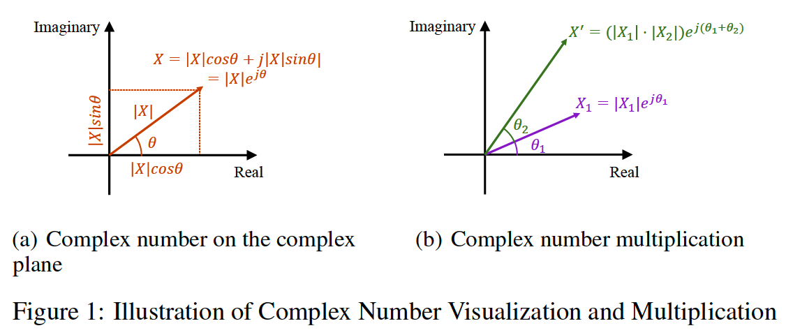
Time Shift & Phase ShiftPermalink

Time Shift = Phase Shift in FREQUENCY domain

• by multiplying a unit complex exponential element with the corresponding space ( in FREQ domain )

Shift signal $x(t)$ forawrd in TIME by $\tau$ = $x(t-\tau)$

$\rightarrow$ Fourier transform: $X_\tau(f)=e^{-j 2 \pi f \tau} X(f)= \mid X(f) \mid e^{j(\theta(f)-2 \pi f \tau)}=[\cos (-2 \pi f \tau)+j \sin (-2 \pi f \tau)] X(f)$

• Amplitude : $\mid X(f) \mid$
• Phase $\theta_\tau(f)=\theta(f)-2 \pi f \tau$
  • linear to the time shift.

(2) FITS PipelinePermalink

(Motivation) Longer TS = Higher frequency resolution

$\rightarrow$ Train FITS to extend TS segment by interpolating the frequency representation of input TS semgnet

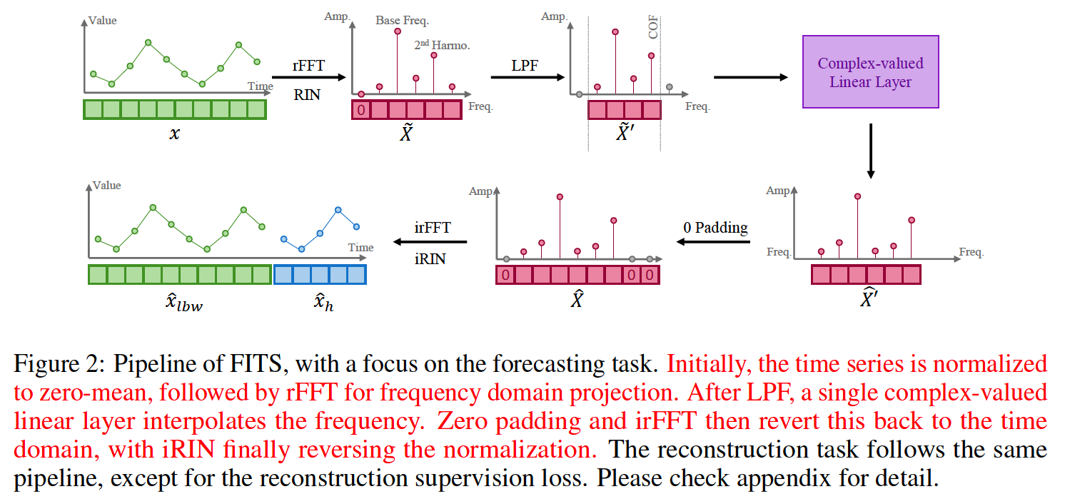
LPF (Low-Pass Filter)

• To reduce the model size
• Eliminates HIGH-frequency components above certain cutoff

Forecasting

• generate the look-back window along with the horizon

  ( = combining backcast & forecast )

Reconstruction

• downsample the original TS based on specific downsampling rate
• then, perform frequency interpolation

(3) Key Mechanism of FITSPermalink

a) Complex Frequency Linear InterpolationPermalink

Interpolation rate: $\eta$

• ratio of the model’s output length $L_o$ to its corresponding input length $L_i$.

Frequency interpolation

• operates on the normalized complex frequency representation ( = half the length of the original TS )

Interpolation rate can also be applied to the frequency domain

• $\eta_{f r e q}=\frac{L_o / 2}{L_i / 2}=\frac{L_o}{L_i}=\eta$.

With an arbitrary frequency $f$ …

• Frequency band $1 \sim f$ in the original signal is linearly projected to the frequency band $1 \sim \eta f$ in the output signal.
• Input length of our complex-valued linear layer = $L$
• Interpolated output length = $\eta L$.

b) Low Pass Filter (LPF)Permalink

• To compress the model’s volume

• By discarding frequency components above a specified cutoff frequency (COF)

• Ensures that a significant portion of the original time series’ meaningful content is preserved

  • High-frequency components filtered out by the LPF typically comprise noise,!

    ( = irrelevant for effective time series modeling )

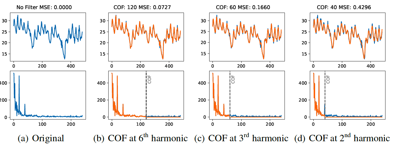
Selecting COF? Nontrivial!

$\rightarrow$ propose method based on the harmonic content of the dominant frequency

Also adopt channel independence

4. ExperimentsPermalink

(1) Forecasting as Frequency InterpolationPermalink

Input Length : $L$ Output Length : $H$ Combination of look-back window & forecasting horizon : $L+H$

Interpolation rate of the forecasting task:

• $\eta_{\text {Fore }}=1+\frac{H}{L}$.