DYffusion; A Dynamics-informed Diffusion Model for Spatio-temporal Forecasting

DYffusion: A Dynamics-informed Diffusion Model for Spatio-temporal Forecasting

Contents

1. Abstract
2. Introduction
3. Background
   1. Problem Setup
   2. Diffusion processes
4. DYffusion: Dynamics-Informed Diffusion Model

Abstract

Dyffusion

• Efficiently training diffusion models for probabilistic spatio-temporal forecasting

• Train a stochastic, time-conditioned interpolator & forecaster network

• Facilitates multi-step & long-range forecasting

• Imposes strong inductive bias & improves computational efficiency

  ( compared to traditional Gaussian noise-based diffusion models )

1. Introduction

Dynamics forecasting = predicting the future behavior of a dynamic system

Generative modeling = promising avenue for probabilistic dynamics forecasting

Challenges in generative modeling

• (1) Computational cost: sequential sampling
• (2) Few methodsd apply diffusion models beyond static images (i.e. Video)

Dyffusion

• Train a dyanmics-informed diffusion model for multi-step probabilistic forecasting
• Non-Gaussian diffusion process
  • relies on temporal interpolation
  • implemented via time-conditioned NN
• Inductive bias by coupling …
  • (1) the diffusion process steps
  • (2) the time steps in the dynamical system

​ \(\rightarrow\) Reduces the computational complexitiy, data efficiency, # of diffusion steps

Contributions

1. Investiage probabilistic spatio-temporal forecasting from the perspective of diffusion
2. Propose DYffusion
   • flexible framework for multi-step forecasting & long-range horizons
   • leverages temporal inductive bias to accelerate training & lower memory needs

2. Background

(1) Problem Setup

Probabilistic spatio-temporal forecasting

Notation

• Dataset of \(\left\{\mathrm{x}_t\right\}_{t=1}^T\) snapshots with \(\mathrm{x}_t \in \mathcal{X}\).
• Task of probabilistic forecasting
  • learn a conditional distribution \(P\left(\mathrm{x}_{t+1: t+h} \mid \mathrm{x}_{t-l+1: t}\right)\)
• Task of forecasting from a single initial condition
  • learn \(P\left(\mathrm{x}_{t+1: t+h} \mid \mathrm{x}_t\right)\).

(2) Diffusion processes

Diffusion step states, \(\mathbf{s}^{(n)}\)

• \(n\) : diffusion step (O), time step (X)

Degradation operator \(D\)

• Add noises
• Input: data point \(\mathbf{s}^{(0)}\)
• Output: \(\mathbf{s}^{(n)}=D\left(\mathbf{s}^{(0)}, n\right)\)
  • for varying degrees of degradation proportional to \(n \in\{1, \ldots, N\}\)
• ex) \(D\) adds Gaussian noise
  • with increasing levels of variance so that \(\mathbf{s}^{(N)} \sim \mathcal{N}(\mathbf{0}, \mathbf{I})\).

Denoising network \(R_\theta\)

• Trained to restore \(\mathbf{s}^{(0)}\), i.e. such that \(R_\theta\left(\mathbf{s}^{(n)}, n\right) \approx \mathbf{s}^{(0)}\).

Diffusion model can be conditioned on the input dynamics by considering \(R_\theta\left(\mathbf{s}^{(n)}, \mathbf{x}_t, n\right)\).

Dynamics forecasting: the diffusion model can be trained to minimize the objective

\(\min _\theta \mathbb{E}_{n \sim \mathcal{U} [ 1, N ], \mathbf{x}_t, \mathbf{s}^{(0)} \sim \mathcal{X}}\left[ \mid \mid R_\theta\left(D\left(\mathbf{s}^{(0)}, n\right), \mathbf{x}_t, n\right)-\mathbf{s}^{(0)} \mid \mid ^2\right]\)…. Eq (1)

• \(\mathbf{s}^{(0)}=\mathbf{x}_{t+1: t+h}\).
• Can be viewed as a generalized version of the standard diffusion models
• (In practice, \(R_\theta\) may be trained to predict the Gaussian noise)

3. DYffusion: Dynamics-Informed Diffusion Model

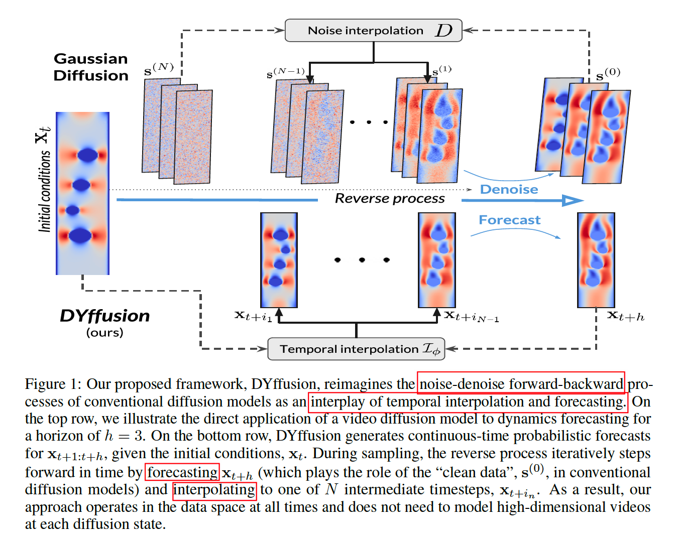
Replace the …

• Degradation operator \(D\) \(\rightarrow\) Stochastic interpolator network \(\mathcal{I}_\phi\)
• Restoration network \(R_\theta\), \(\rightarrow\) Deterministic forecaster network \(F_\theta\).

HIGH level: time step (temporal dynamics in data)

LOW level: diffusion step

• intermediate steps in the diffusion process can be reused as forecasts for actual timesteps in multi-step forecasting

Advantage

• Diffusion) initialized with the initial conditions of the dynamics
• Standard) designed for unconditional generation & reverse from WN … more diffusion steps!

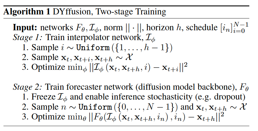
a) “Temporal Interpolation” = FORWARD process

To impose temporal bias, train a time-conditioned network \(\mathcal{I}_\phi\) to interpolate between snapshots of data.

Goal

• given a horizon \(h\)
• train \(\mathcal{I}_\phi\) so that \(\mathcal{I}_\phi\left(\mathbf{x}_t, \mathbf{x}_{t+h}, i\right) \approx \mathbf{x}_{t+i}\) for \(i \in\{1, \ldots, h-1\}\)

Loss function

• \(\min _\phi \mathbb{E}_{i \sim \mathcal{U} [ 1, h-1 ], \mathbf{x}_{t, t+i, t+h} \sim \mathcal{X}}\left[ \mid \mid \mathcal{I}_\phi\left(\mathbf{x}_t, \mathbf{x}_{t+h}, i\right)-\mathbf{x}_{t+i} \mid \mid ^2\right]\).

Interpolation = Easier task than forecasting

\(\rightarrow\) Use the interpolator \(\mathcal{I}_\phi\) during inference to interpolate beyond the temporal resolution of the data

Stochastic interpolator

• To generate probabilistic forecasts
• Produce stochastic outputs within the diffusion model and during inference time
  • by Monte Carlo dropout at inference time.

b) “Forecasting” = REVERSE process

Interpolator network, \(\mathcal{I}_\phi\), is frozen with inference stochasticity enabled

Loss function

• \(\min _\theta \mathbb{E}_{n \sim \mathcal{U} [] 0, N-1 ], \mathbf{x}_{t, t+h} \sim \mathcal{X}}\left[ \mid \mid F_\theta\left(\mathcal{I}_\phi\left(\mathbf{x}_t, \mathbf{x}_{t+h}, i_n \mid \xi\right), i_n\right)-\mathbf{x}_{t+h} \mid \mid ^2\right]\).

To include the setting where \(F_\theta\) learns to forecast the initial conditions, we define \(i_0:=0\) and \(\mathcal{I}_\phi\left(\mathrm{x}_t, \cdot, i_0\right):=\mathbf{x}_t\).

Additional loss

• Problem) \(\mathcal{I}_\phi\) is frozen in the second stage & imperfect forecasts \(\hat{\mathbf{x}}_{t+h}=\) \(F_\theta\left(\mathcal{I}_\phi\left(\mathrm{x}_t, \mathrm{x}_{t+h}, i_n\right), i_n\right)\) may degrade accuracy when sequential sampling
• Solution) introduce a one-step look-ahead loss term
  • \(\mid \mid F_\theta\left(\mathcal{I}_\phi\left(\mathbf{x}_t, \hat{\mathbf{x}}_{t+h}, i_{n+1}\right), i_{n+1}\right)-\mathbf{x}_{t+h} \mid \mid ^2\) whenever \(n+1<N\) .
  • Weight the two loss terms equally.

Additionally, providing a clean or noised form of the initial conditions \(\mathbf{x}_t\) as an additional input to the forecaster net can improve performance

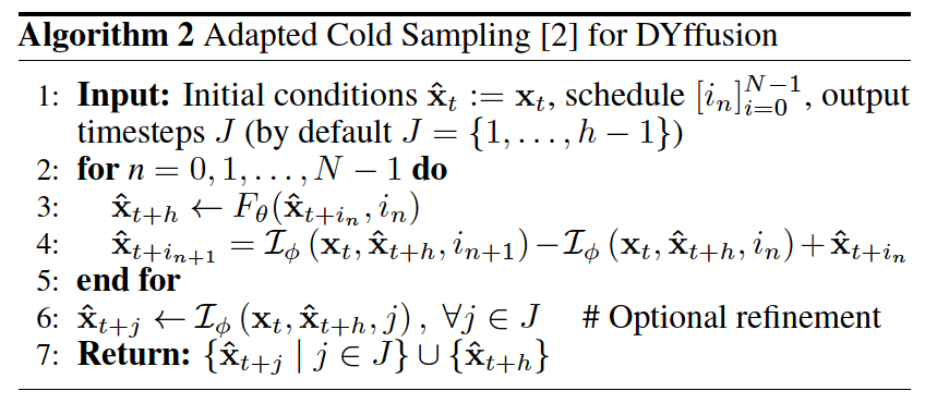
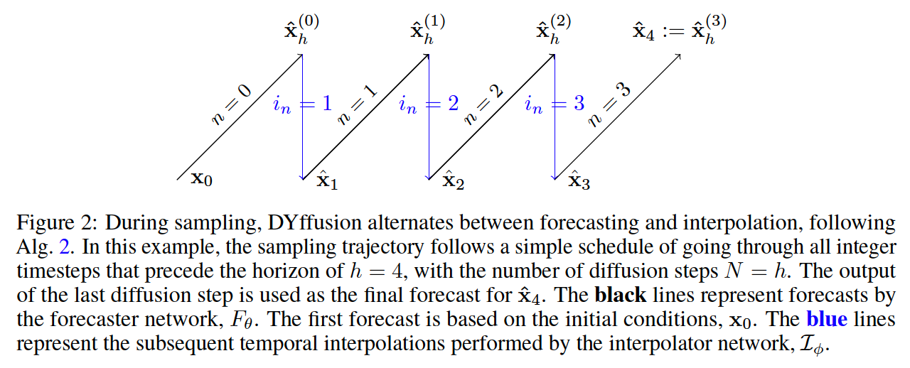
c) Sampling

\(p_\theta\left(\mathbf{s}^{(n+1)} \mid \mathbf{s}^{(n)}, \mathbf{x}_t\right)= \begin{cases}F_\theta\left(\mathbf{s}^{(n)}, i_n\right) & \text { if } n=N-1 \\ \mathcal{I}_\phi\left(\mathbf{x}_t, F_\theta\left(\mathbf{s}^{(n)}, i_n\right), i_{n+1}\right) & \text { otherwise, }\end{cases}\).

• \(\mathbf{s}^{(0)}=\mathbf{x}_t\) : initial conditions
• \(\mathbf{s}^{(n)} \approx \mathbf{x}_{t+i_n}\) : predictions of intermediate steps

\(n=0\) : Start of the reverse process (i.e. \(\mathbf{x}_t\) ),

\(n=N\) : Final output of the reverse process (here, \(\mathbf{x}_{t+h}\) )

d) Memory Footprint

DYffusion

• requires only \(\mathbf{x}_t\) and \(\mathbf{x}_{t+h}\) (plus \(\mathbf{x}_{t+i}\) during the first stage) to train

Direct multi-step prediction models

• require \(\mathbf{x}_{t: t+h}\) to compute the loss

  ( must fit \(h+1\) timesteps of data into memory, which scales poorly with the forecasting horizon \(h\) )

e) Reverse process as ODE.

DYffusion models the dynamics as

• \(\frac{d \mathbf{x}(s)}{d s}=\frac{d \mathcal{I}_\phi\left(\mathbf{x}_t, F_\theta(\mathbf{x}, s), s\right)}{d s}\).

During prediction,

• \(\mathbf{x}(s)=\mathbf{x}(t)+\int_t^s \frac{d \mathcal{I}_\phi\left(\mathbf{x}_t, F_\theta(\mathbf{x}, s), s\right)}{d s} d s \quad \text { for } s \in(t, t+h]\).
• The initial condition is given by \(\mathbf{x}(t)=\mathbf{x}_t\).