PriSTI; A Conditional Diffusion Framework for Spatiotemporal Imputation

PriSTI; A Conditional Diffusion Framework for Spatiotemporal Imputation

Contents

1. Abstract
2. Introduction
3. Preliminaries
4. Methodology
   1. Diffusion Model for Spatiotemporal Imputation
   2. Design of Noise Prediction Model
      1. Conditional Feature Extraction Module
      2. Noise Estimation Module
      3. Auxiliary Information and Output

0. Abstract

Task: Spatiotemporal Imputation

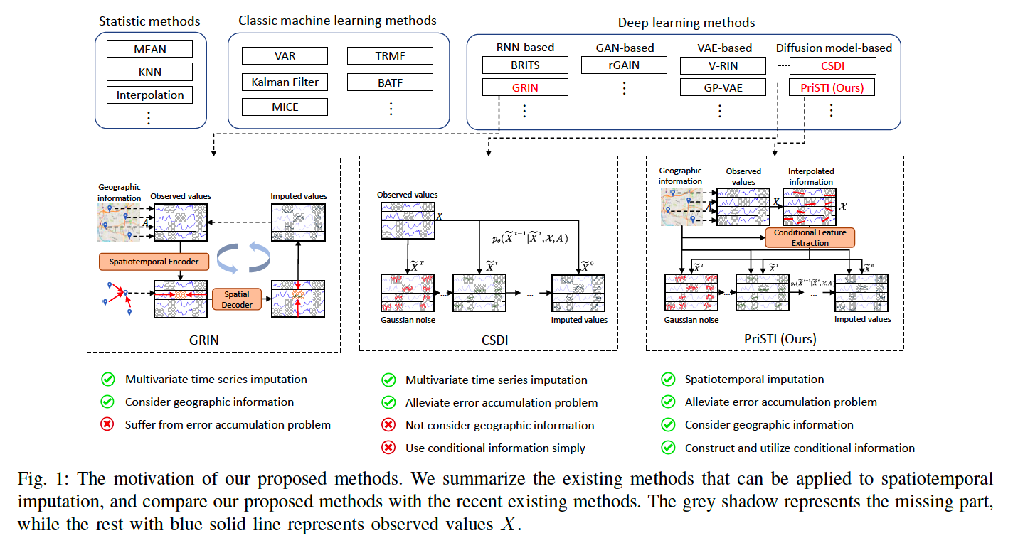
Previous works

• (1) Autoregressive:
  • Limitation) suffer from error accumulation
• (2) DDPM based:
  • impute missing values, conditioned by observations
  • avoid inferring missing values from inaccurate historical imputation
  • Limitation) construction & utilization of conditional information are challenges

Propose PriSTI

• Conditional diffusion for spatiotemporal imputation with enhanced prior modeling
• Framework
  • (1) Conditional feature extraction
    • extract coarse & effective spatiotemporal dependencies
  • (2) Noise estimation module
    • using spatiotemporal attention weights calculated by conditional feature

1. Introduction

Problem of applying diffusion to impuation:

\(\rightarrow\) Modeling & introducing of condittional information in diffusion models are inevitable

• ex) spatiotemporal imputation: construction of conditional information with spatiotemporal dependencies

Limitation of CSDI

• (1) Only considers temporal & feature dependencies

  \(\rightarrow\) Does not consider spatial similarity (i.e. geographic proximity)

• (2) Combine the condition info & perturbed values directly

  \(\rightarrow\) Lead to inconsistency inside the input spatiotemporal data

\(\rightarrow\) Solution: PriSTI

PriSTI

Conditional diffusion framework for SpatioTemporal Imputation with enhanced Prior modeling

Main Challenge of applying diffusion to spatiotemporal imputation:

• How to model & utilize spatiotemporal depenencies in conditional information

\(\rightarrow\) PriSTI: by extracting conditional feature from observation as a global context probior

Input

• (1) Observed spatiotemporal data
• (2) Geographical information

Training

• Step 1) Observed values are randomly erased ( = become imputation target )

• Step 2) Interpolate incomplete data

• Step 3) Conditional feature exztraction module

  • use both spatiotemporal global features & geographic information

• Step 4) Noise estimation module

  • utilize the above conditional information

    ( use conditional feature as the global context prior, to calculate spatiotemporal attention weight )

Contribution

1. PrisTI: constructs & utilizes conditional inforamation with (1) spatiotemporal global correlations & (2) geographic relationships
2. Specialized noise prediction model that exgracts conditional features
   • from enhanced observations,
   • calculating the spatiotemporal attention weights using the extracted global context prior

2. Preliminaries

(1) Spatiotemporal Data

\[X_{1: L}=\left\{X_1, X_2, \cdots, X_L\right\} \in \mathbb{R}^{N \times L}\]

• \(X_l \in \mathbb{R}^N\) is the values observed at time \(l\) by \(N\) observation nodes

Binary mask \(M_l \in\{0,1\}^N\)

• to represent the observed mask at time \(l\)
• where \(m_l^{i, j}=1\) represents the value is observed

Manual binary mask \(\widetilde{M} \in \mathbb{R}^{N \times L}\).

• Manually select the imputation target \(\widetilde{X} \in \mathbb{R}^{N \times L}\) for training and evaluation

(2) Adjacency matrix

Cnsider the setting of static graph, i.e., the geographic information \(A\) does not change over time.

(3) Problem Statement

Given the (1) incomplete observed spatiotemporal data \(X\) and (2) geographical information \(A\)

\(\rightarrow\) Estimate the missing values or corresponding distributions in spatiotemporal data \(X_{1: L}\).

(4) DDPM

\(\widetilde{X}^0 \sim p_{\text {data }}\) .

\(\widetilde{X}^T \sim \mathcal{N}(0, \boldsymbol{I})\) .

3. Methodology

Adopts a conditional diffusion framework to exploit

• (1) spatiotemporal global correlation
• (20 geographic relationships

Specialized noise prediction model

• to enchance & extract the conditional feature

(1) Diffusion Model for Spatiotemporal Imputation

Reverse process : conditioned on the

• (1) Interpolated conditional information \(\mathcal{X}\)
  • that enhances the observed values
• (2) Geographical information \(A\).

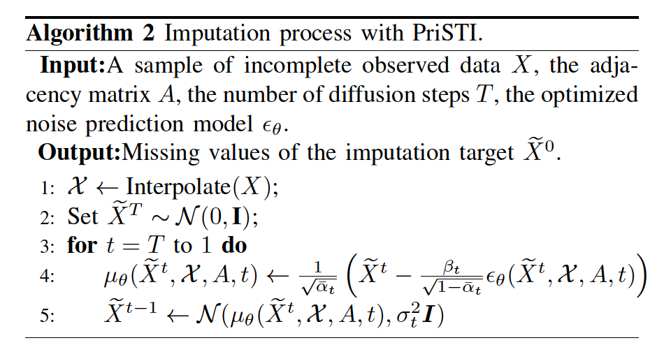
\(\begin{aligned} & p_\theta\left(\widetilde{X}^{0: T-1} \mid \tilde{X}^T, \mathcal{X}, A\right)=\prod_{t=1}^T p_\theta\left(\widetilde{X}^{t-1} \mid \tilde{X}^t, \mathcal{X}, A\right), \\ & p_\theta\left(\widetilde{X}^{t-1} \mid \tilde{X}^t, \mathcal{X}, A\right)=\mathcal{N}\left(\widetilde{X}^{t-1} ; \mu_\theta\left(\widetilde{X}^t, \mathcal{X}, A, t\right), \sigma_t^2 \boldsymbol{I}\right) \end{aligned}\).

\(\begin{aligned} & \mu_\theta\left(\tilde{X}^t, \mathcal{X}, A, t\right)=\frac{1}{\sqrt{\bar{\alpha}_t}}\left(\tilde{X}^t-\frac{\beta_t}{\sqrt{1-\bar{\alpha}_t}} \epsilon_\theta\left(\tilde{X}^t, \mathcal{X}, A, t\right)\right) \\ & \sigma_t^2=\frac{1-\bar{\alpha}_{t-1}}{1-\bar{\alpha}_t} \beta_t \end{aligned}\).

• \(\epsilon_\theta\) :Noise prediction model
• Input
  • Noisy sample \(\tilde{X}^t\)
  • Conditional information \(\mathcal{X}\)
  • Adjacency matrix \(A\)

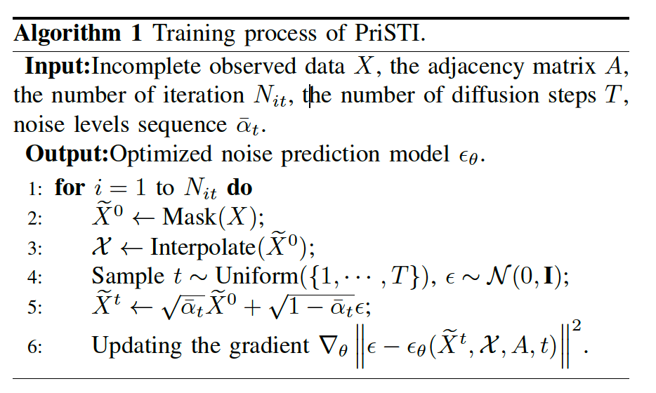
a) Training Process

Mask the input observed value \(X\)

\(\rightarrow\) Obtain the imputation target \(\widetilde{X}^t\),

\(\mathcal{L}(\theta)=\mathbb{E}_{\tilde{X}^0 \sim q\left(\tilde{X}^0\right), \epsilon \sim \mathcal{N}(0, I)} \mid \mid \epsilon-\epsilon_\theta\left(\tilde{X}^t, \mathcal{X}, A, t\right) \mid \mid ^2\).

• Imputation target \(\widetilde{X}^0\)
• Interpolated conditional information \(\mathcal{X}\),

b) Imputation Process

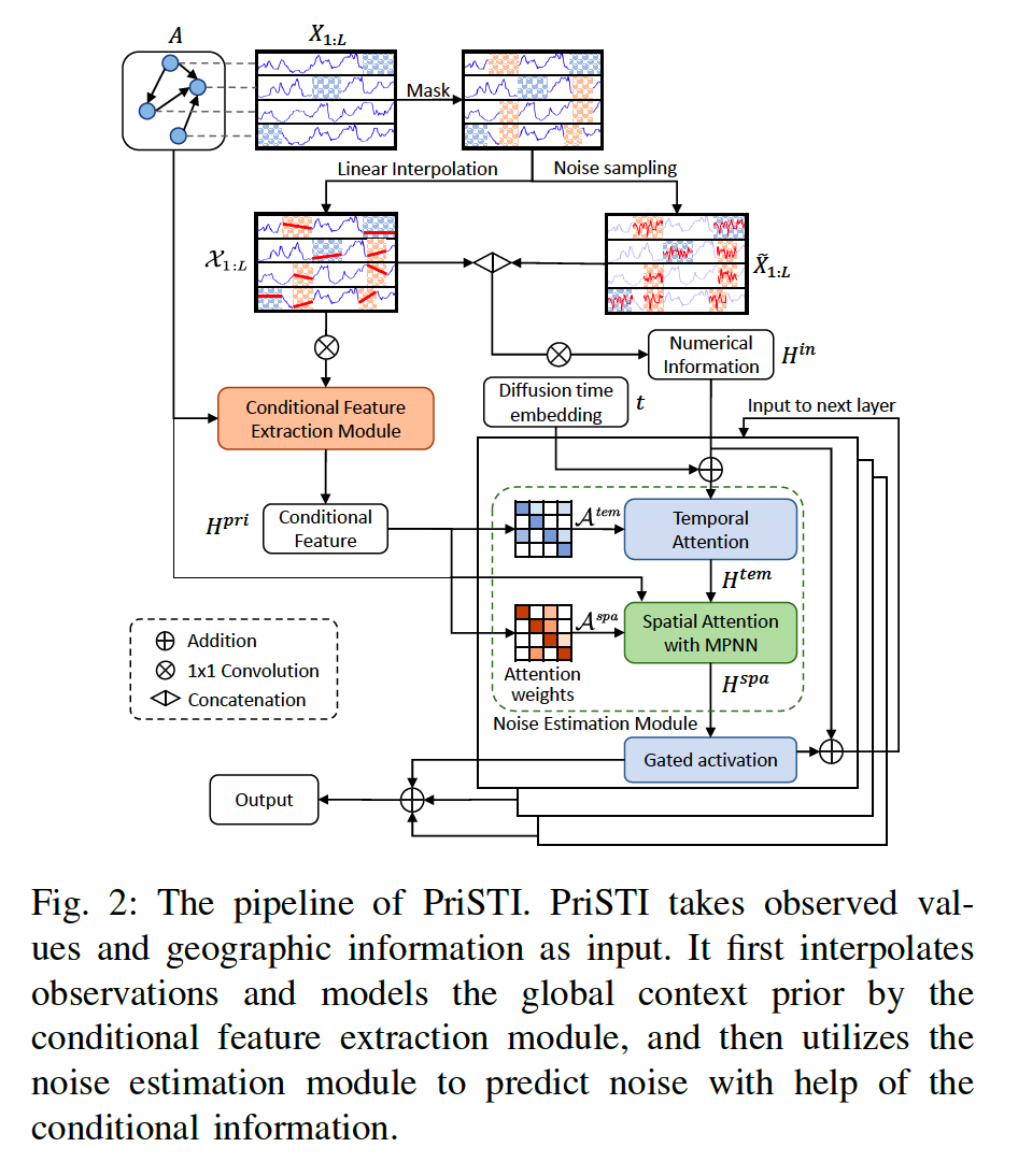
(2) Design of Noise Prediction Model

Noise prediction model \(\epsilon_\theta\) for spatiotemporal imputation

Procedures

• Step 1) Interpolate the observed value
  • to obtain the enhanced coarse conditional information
• Step 2) Conditional feature extraction module
  • to model the spatiotemporal correlation
  • Using the coarse interpolation result
• Step 3) Noise estimation module
  • utilize extracted feature, which provides global context prior

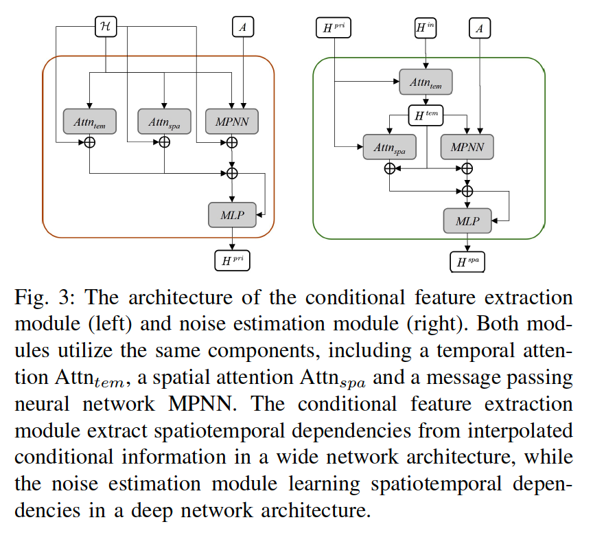
a) Conditional Feature Extraction Module

CSDI: regards the observed values as conditional information

However …. unstable!

\(\rightarrow\) enhance the observed values, by applying linear interpolation

Linear interpolation

• based on temporal continuity
• does not introeuce randomness
• retain certain spatiotemporal consistency
• fast computation

\(\rightarrow\) Only simply describes the linear uniform change in time

\(\rightarrow\) \(\therefore\) Design a learnable module \(\gamma(\cdot)\) o model a conditional feature \(H^{p r i}\) with spatiotemporal information as a global context prior

Conditional Feature Extraction Module \(\gamma(\cdot)\)

• Input:

  • Interpolated conditional information \(\mathcal{X}\)
  • Adjacency matrix \(A\)

• Extract:

  • Spatiotemporal dependencies from \(\mathcal{X}\)

• Output:

  • \(H^{p r i}\) as the global context

    \(\rightarrow\) used for the calculation of spatiotemporal attention weights

  • \(H^{\text {pri }}=\gamma(\mathcal{H}, A)\),

    • where \(\mathcal{H}=\operatorname{Conv}(\mathcal{X})\) and \(\mathcal{H} \in \mathbb{R}^{N \times L \times d}\), and \(d\) is the channel size.

Adopt the graph convolution module from Graph Wavenet

b) Noise Estimation Module

Inputs of the noise estimation module include two parts

• (1) Noisy information \(H^{i n}=\operatorname{Conv}\left(\mathcal{X} \mid \mid \widetilde{X}^t\right)\)
  • consists of interpolation information \(\mathcal{X}\) and noise sample \(\widetilde{X}^t\),
• (2) Prior information
  • (2-1) Conditional feature \(H^{p r i}\)
  • (2-2) Adjacency matrix \(A\).

(Details)

• Temporal features \(H^{\text {tem }}\) are first learned through a temporal dependency learning module \(\gamma_{\mathcal{T}}(\cdot)\), and then the temporal features are aggregated through a spatial dependency learning module \(\gamma_{\mathcal{S}}(\cdot)\).

• When the number of nodes in the spatiotemporal data is large, the computational cost of spatial global attention is high

  \(\rightarrow\) map \(N\) nodes to \(k\) virtual nodes, where \(k<N\).

c) Auxiliary Information and Output

Add auxiliary information \(U=\operatorname{MLP}\left(U_{\text {tem }}, U_{\text {spa }}\right)\)

• to both the conditional feature extraction module and the noise estimation module
• \(U_{t e m}\) :the sine-cosine temporal encoding
• \(U_{s p a}\) : learnable node embedding