Consistency Models

Consistency Models

Contents

1. Abstract
2. sIntroduction
3. Diffusion Model
4. CD
5. CT

Abstract

Limitation of diffusion models

• depend on iterative sampling process \(\rightarrow\) slow generation

Consistency models

• New family of models that generate high quality samples, by directly mapping noise to data

• Fast one-step generation by design

  ( still allowing multistep sampling to trade compute for sample quality )

• Zero-shot data editing
  • ex) image inpainting, colorization, and super-resolution, without requiring explicit training
• Can be trained either by …
  • (1) distilling pre-trained diffusion models
  • (2) standalone generative models
• Experiments
  • outperform existing distillation techniques for diffusion models in one- and few-step sampling

1. Introduction

Goal: Create generative models that facilitate efficient, single-step generation without sacrificing important advantages of iterative sampling & performing zero-shot data editing tasks

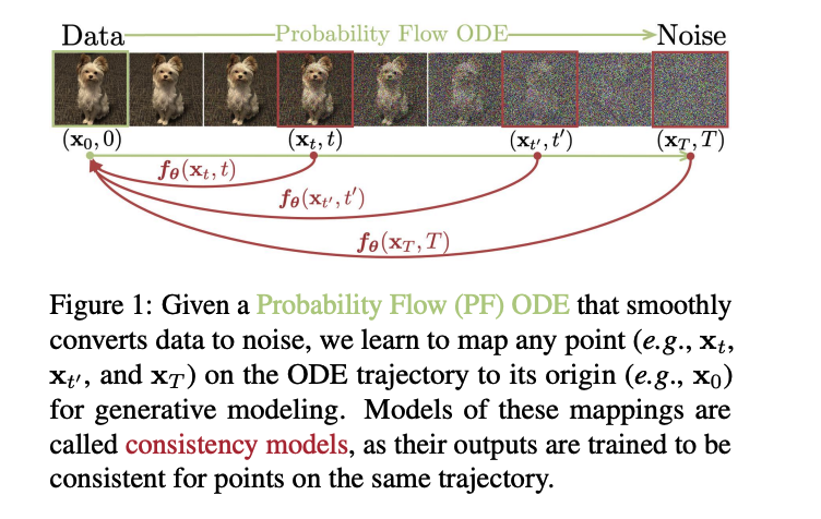
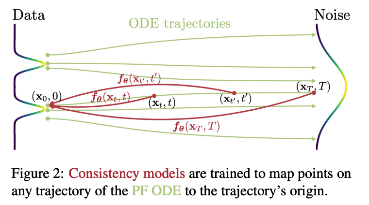
• build on top of the probability flow (PF) ordinary differential equation (ODE) in continuous-time diffusion models (Song et al., 2021)
  • trajectories smoothly transition the data distribution into a tractable noise distribution
• learn a model that maps any point at any time step to the trajectory’s starting point

Consistency Model

• Self-consistency:
  • points on the same trajectory map to the “same initial point”

• Generate data samples (initial points of ODE trajectories, e.g., \(x_0\))

  by converting random noise vectors (end points of ODE trajectories, e.g., \(x_T\))

  with only ONE network evaluation.

• Also allows multi-step

  • By chaining the outputs of consistency models at multiple time steps, can improve sample quality

    & perform zero-shot data editing ( at the cost of more compute )

Training consistency model: 2 methods based on enforcing the self-consistency

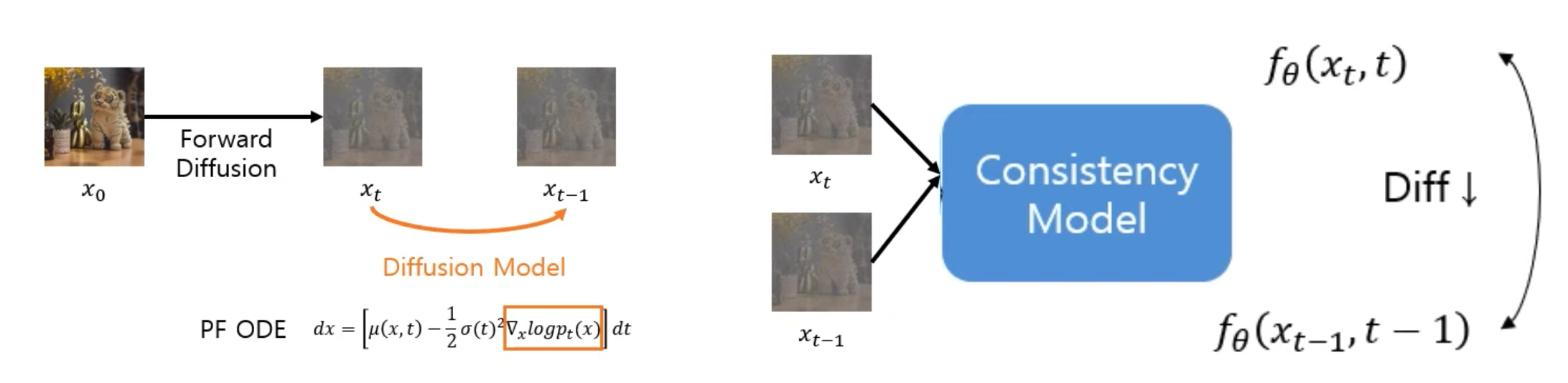
• (1) Consistency Distillation (CD): with pretrained diffusion model
  • Generate pairs of adjacent points on a PF ODE trajectory.
  • By minimizing the difference between model outputs for these pairs, effectively distill a diffusion model into a consistency model
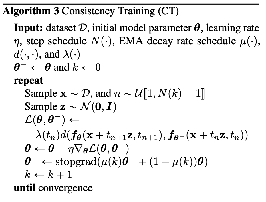
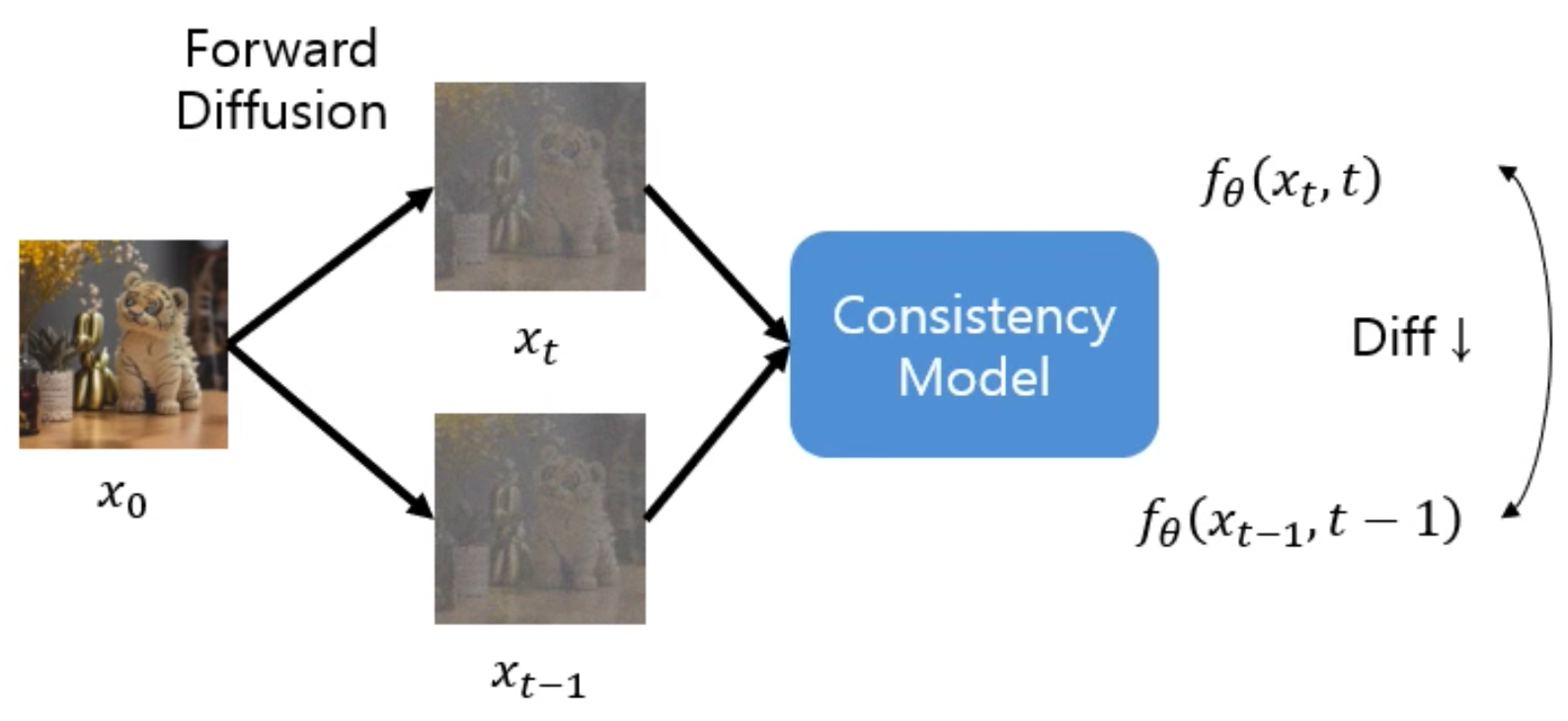
• (2) Consistency Training (CT): w/o pretrained diffusion model
  • Train a consistency model in isolation.
  • situates consistency models as an independent family of generative models

\(\rightarrow\) Neither requires adversarial training!

Consistency Distillation (CD)

Consistency Training (CT)

2. Diffusion Model

By progressively perturbing data to noise via Gaussian perturbations

& Creating samples from noise via sequential denoising steps

(1) SDE & PF-ODE

• SD: Stochastic Differential Equation
• PF-ODE: Probability Flow - Oridnary Differential equation

[SDE]

\(\mathrm{d} \mathbf{x}_t=\boldsymbol{\mu}\left(\mathbf{x}_t, t\right) \mathrm{d} t+\sigma(t) \mathrm{d} \mathbf{w}_t\).

Remarkable property of SDE

• Existence of an ODE, dubbed the Probability Flow (PF) \(\rightarrow\) PF-ODE

[PF-ODE]

\(\mathrm{d} \mathbf{x}_t=\left[\boldsymbol{\mu}\left(\mathbf{x}_t, t\right)-\frac{1}{2} \sigma(t)^2 \nabla \log p_t\left(\mathbf{x}_t\right)\right] \mathrm{d} t\)…. Eq (a)

Details: SDE is designed such that \(p_T(\mathbf{x})\) is close to a tractable Gaussian distribution \(\pi(\mathbf{x})\).

• \(\boldsymbol{\mu}(\mathbf{x}, t)=\mathbf{0}\) and \(\sigma(t)=\sqrt{2 t}\)

  \(\rightarrow\) we have \(p_t(\mathbf{x})=p_{\text {data }}(\mathbf{x}) \otimes \mathcal{N}\left(\mathbf{0}, t^2 \boldsymbol{I}\right)\), and \(\pi(\mathbf{x})=\mathcal{N}\left(\mathbf{0}, T^2 \boldsymbol{I}\right)\).

Procedures

• Step 1) Train a score model \(s_\phi(\mathbf{x}, t) \approx \nabla \log p_t(\mathbf{x})\) via score matching

• Step 2) Plug it into Eq (a) to obtain an empirical estimate of the PF ODE

  • takes the form of \(\frac{\mathrm{d} \mathbf{x}_t}{\mathrm{~d} t}=-t s_\phi\left(\mathbf{x}_t, t\right)\)….. empirical PF-ODE

• Step 3) Sample \(\hat{\mathbf{x}}_T \sim \pi=\mathcal{N}\left(\mathbf{0}, T^2 \boldsymbol{I}\right)\)

  • to initialize the empirical PF ODE

• Step 4) Solve it backwards in time with any numerical ODE solver to obtain the solution trajectory \(\left\{\hat{\mathbf{x}}_t\right\}_{t \in[0, T]}\).

  \(\rightarrow\) Resulting \(\hat{\mathbf{x}}_0\) can then be viewed as an approximate sample from \(p_{\text {data }}(\mathbf{x})\).

Bottleneck of Diffusion Models

Slow sampling speed

ODE solvers

• requires iterative evaluations of the score model \(s_\phi(\mathbf{x}, t)\),

Other techniques

• Faster numerical ODE solvers
• Distillation techniques

\(\rightarrow\) [ODE] Still need more than 10 evaluation steps to generate competitive samples

\(\rightarrow\) [Distillation] Rely on collecting a large dataset of samples from the diffusion model prior to distillation

3. Consistency Models

[Consistency Function] \(\boldsymbol{f}:\left(\mathbf{x}_t, t\right) \mapsto \mathbf{x}_\epsilon\).

• Solution trajectory \(\left\{\mathbf{x}_t\right\}_{t \in[\epsilon, T]}\) of the PF ODE

• Self-consistency:

  • Outputs are consistent for arbitrary pairs of \(\left(\mathbf{x}_t, t\right)\) that belong to the same PF ODE trajectory

    ( i.e., \(\boldsymbol{f}\left(\mathbf{x}_t, t\right)=\boldsymbol{f}\left(\mathbf{x}_{t^{\prime}}, t^{\prime}\right)\) for all \(t, t^{\prime} \in[\epsilon, T]\). )

• Similar definition is used for neural flows in the context of neural ODEs

  ( \(\leftrightarrow\) Compared to neural flows, consistency models do not need to be invertible )

Boundary condition

For any consistency function \(\boldsymbol{f}(\cdot, \cdot)\), \(\boldsymbol{f}\left(\mathbf{x}_\epsilon, \epsilon\right)=\mathbf{x}_\epsilon\), i.e., \(\boldsymbol{f}(\cdot, \epsilon)\) is an identity function

• Also the most confining architectural constraint on consistency models

( Method 1 )

\(\boldsymbol{f}_{\boldsymbol{\theta}}(\mathbf{x}, t)= \begin{cases}\mathbf{x} & t=\epsilon \\ F_{\boldsymbol{\theta}}(\mathbf{x}, t) & t \in(\epsilon, T]\end{cases}\).

( Method 2 )

\(\boldsymbol{f}_{\boldsymbol{\theta}}(\mathbf{x}, t)=c_{\text {skip }}(t) \mathbf{x}+c_{\text {out }}(t) F_{\boldsymbol{\theta}}(\mathbf{x}, t)\).

• where \(c_{\text {skip }}(t)\) and \(c_{\text {out }}(t)\) are differentiable functions s.t \(c_{\text {skip }}(\epsilon)=1\), and \(c_{\text {out }}(\epsilon)=0\).

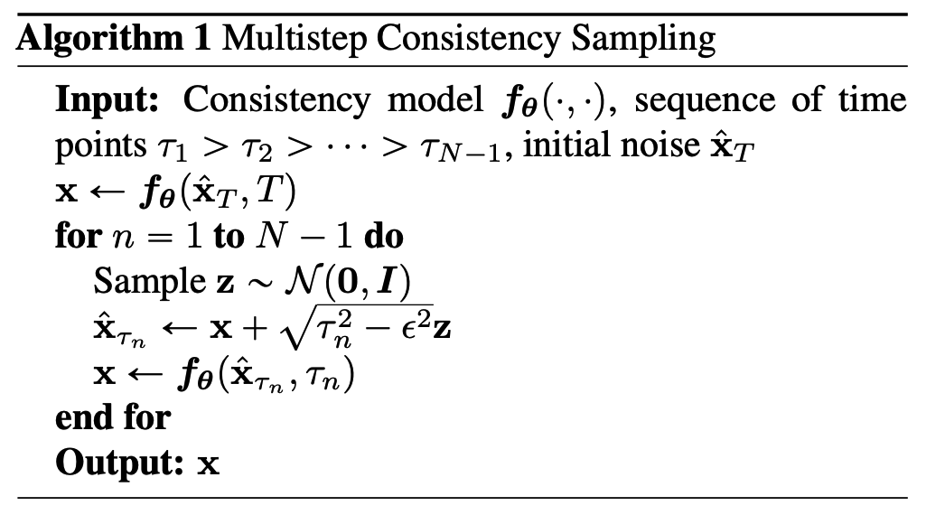
Sampling

With a well-trained consistency model \(\boldsymbol{f}_{\boldsymbol{\theta}}(\cdot, \cdot)\), generate samples by sampling from the initial distribution \(\hat{\mathbf{x}}_T \sim \mathcal{N}\left(\mathbf{0}, T^2 \boldsymbol{I}\right)\)

\(\rightarrow\) \(\hat{\mathbf{x}}_\epsilon=\boldsymbol{f}_{\boldsymbol{\theta}}\left(\hat{\mathbf{x}}_T, T\right)\).

• Only ONE forward pass through the consistency model
• Can also evaluate the consistency model multiple times

4. Training Consistency Models via Distillation

Training consistency models based on distilling a pre-trained score model \(s_\phi(\mathbf{x}, t)\).

\(\rightarrow\) Plugging the score model \(s_\phi(\mathbf{x}, t)\) into the PF ODE.

Discretize the time horizon \([\epsilon, T]\) into \(N-1\) sub-intervals

• with boundaries \(t_1=\epsilon<\) \(t_2<\cdots<t_N=T\). I

When \(N\) is sufficiently large, can obtain an accurate estimate of \(\mathbf{x}_{t_n}\) from \(\mathbf{x}_{t_{n+1}}\)

( by running one discretization step of a numerical ODE solver )

• \(\hat{\mathbf{x}}_{t_n}^{\boldsymbol{\phi}}:=\mathbf{x}_{t_{n+1}}+\left(t_n-t_{n+1}\right) \Phi\left(\mathbf{x}_{t_{n+1}}, t_{n+1} ; \boldsymbol{\phi}\right)\).

  • \(\Phi(\cdots ; \phi)\) : update function of a onestep ODE solver applied to the empirical PF ODE.

    • ex) Euler solver, we have \(\Phi(\mathbf{x}, t ; \boldsymbol{\phi})=\) \(-t s_\phi(\mathbf{x}, t)\)

      \(\rightarrow\) \(\hat{\mathbf{x}}_{t_n}^\phi=\mathbf{x}_{t_{n+1}}-\left(t_n-t_{n+1}\right) t_{n+1} s_\phi\left(\mathbf{x}_{t_{n+1}}, t_{n+1}\right)\)

Procedures

• Step 1) Given a data point \(\mathbf{x}\), generate a pair of adjacent data points \(\left(\hat{\mathbf{x}}_{t_n}^\phi, \mathbf{x}_{t_{n+1}}\right)\) on the PF ODE trajectory
• Step 2) Train the consistency model by minimizing its output differences on the pair \(\left(\hat{\mathbf{x}}_{t_n}^\phi, \mathbf{x}_{t_{n+1}}\right)\).

\(\mathcal{L}_{C D}^N\left(\boldsymbol{\theta}, \boldsymbol{\theta}^{-} ; \boldsymbol{\phi}\right):= \quad \mathbb{E}\left[\lambda\left(t_n\right) d\left(\boldsymbol{f}_{\boldsymbol{\theta}}\left(\mathbf{x}_{t_{n+1}}, t_{n+1}\right), \boldsymbol{f}_{\boldsymbol{\theta}^{-}}\left(\hat{\mathbf{x}}_{t_n}^\phi, t_n\right)\right)\right]\).

\(\boldsymbol{\theta}^{-} \leftarrow \operatorname{stopgrad}\left(\mu \boldsymbol{\theta}^{-}+(1-\mu) \boldsymbol{\theta}\right)\).

5. Training Consistency Models in Isolation

Avoid pre-trained score model by leveraging the following unbiased estimator

\(\nabla \log p_t\left(\mathbf{x}_t\right)=-\mathbb{E}\left[\frac{\mathbf{x}_t-\mathbf{x}}{t^2} \mid \mathbf{x}_t\right]\).

• where \(\mathbf{x} \sim p_{\text {data }}\) and \(\mathbf{x}_t \sim \mathcal{N}\left(\mathbf{x} ; t^2 \boldsymbol{I}\right)\).

\(\rightarrow\) Given \(\mathbf{x}\) and \(\mathbf{x}_t\), we can estimate \(\nabla \log p_t\left(\mathbf{x}_t\right)\) with \(-\left(\mathbf{x}_t-\mathbf{x}\right) / t^2\).