Modeling Temporal Data as Continuous Functions with Stochastic Process Diffusion

Modeling Temporal Data as Continuous Functions with Stochastic Process Diffusion

Contents

1. Abstract

Abstract

Temporal data = discretized measurements of the underlying function

To build a generative model … need to model the stochastic process that governs it.

\(\rightarrow\) Solution: Define the denoising diffusion model in the function space, which also allows us to naturally handle irregularly-sampled observations.

Details

• Define suitable noise sources

• Introduce novel denoising and score-matching models

Experiments

• MTS probabilistic forecasting and imputation
• Can be interpreted as a neural process.

1. Introduction

Diffusion for data measured in continuous time

= by treating it as a discretization of some continuous function.

Instead of adding noise to each DATA POINT independently,

we add the noise to the WHOLE FUNCTION while preserving its continuity.

In Section 3, we show that this can be done by using stochastic processes as noise generators

Final noisy function = sample from a known stochastic process

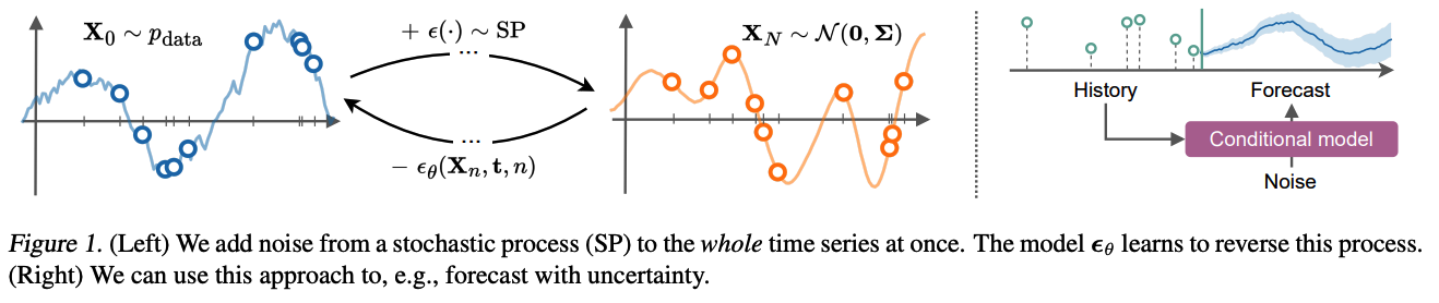
• Data = set of (irregularly-sampled) points that correspond to some underlying function
• [Forward] Add noise to this function \(\rightarrow\) reach the prior stochastic process.
• [Backward] Generate new function samples.

2. Background

Notation

• Training data \(\left\{\boldsymbol{x}_i\right\}\), with \(\boldsymbol{x}_i \in \mathbb{R}^d\)
• Goal of generative modeling : learn \(p(\boldsymbol{x})\) & generate new samples

Brief overview of the two ways to define diffusion

• (1) Noise is added across \(N\) increasing scales
• (2) Stochastic differential equation (SDE)

(1) Fixed-step diffusion

Denoising diffusion probabilistic model (DDPM)

• gradually adds fixed Gaussian noise to \(\boldsymbol{x}_0\) via known scales \(\beta_n\)
  • progressively noisier values \(\boldsymbol{x}_1, \boldsymbol{x}_2, \ldots, \boldsymbol{x}_N\). …. \(\boldsymbol{x}_N \sim \mathcal{N}(\mathbf{0}, \boldsymbol{I})\)
  • sequence of positive noise (variance) scales \(\beta_1, \ldots, \beta_N\) has to be increasing
• \(q\left(\boldsymbol{x}_n \mid \boldsymbol{x}_{n-1}\right)=\mathcal{N}\left(\sqrt{1-\beta_n} \boldsymbol{x}_{n-1}, \beta_n \boldsymbol{I}\right)\).
• \(q\left(\boldsymbol{x}_n \mid \boldsymbol{x}_0\right)=\mathcal{N}\left(\sqrt{\bar{\alpha}_n} \boldsymbol{x}_0,\left(1-\bar{\alpha}_n\right) \boldsymbol{I}\right)\).
  • \(\alpha_n=1-\beta_n\) and \(\bar{\alpha}_n=\prod_{k=1}^n \alpha_k\),

• \(q\left(\boldsymbol{x}_{n-1} \mid \boldsymbol{x}_n, \boldsymbol{x}_0\right)=\mathcal{N}\left(\tilde{\boldsymbol{\mu}}_n, \tilde{\beta}_n \boldsymbol{I}\right)\). - \(\tilde{\boldsymbol{\mu}}_n=\frac{\sqrt{\bar{\alpha}_{n-1}} \beta_n}{1-\bar{\alpha}_n} = \boldsymbol{x}_0+\frac{\sqrt{\alpha_n}\left(1-\bar{\alpha}_{n-1}\right)}{1-\bar{\alpha}_n} \boldsymbol{x}_n\). - \(\tilde{\beta}_n=\frac{1-\bar{\alpha}_{n-1}}{1-\bar{\alpha}_n} \beta_n\).

• Loss: \(\mathcal{L}=\mathbb{E}_{\boldsymbol{\epsilon}, n}\left[ \mid \mid \boldsymbol{\epsilon}_\theta\left(\sqrt{\bar{\alpha}_n} \boldsymbol{x}_0+\sqrt{1-\bar{\alpha}_n} \boldsymbol{\epsilon}, n\right)-\boldsymbol{\epsilon} \mid \mid _2^2\right]\).

(2) Score-based SDE

Continuous diffusion of vector valued data, \(\boldsymbol{x}_0 \mapsto \boldsymbol{x}_s\)

• where \(s \in[0, S]\) … continuous variable.

Forward: \(\mathrm{d} \boldsymbol{x}_s=f\left(\boldsymbol{x}_s, s\right) \mathrm{d} s+g(s) \mathrm{d} W_s\).

Reverse: \(\mathrm{d} \boldsymbol{x}_s=\left[f\left(\boldsymbol{x}_s, s\right)-g(s)^2 \nabla_{\boldsymbol{x}_s} \log p\left(\boldsymbol{x}_s\right)\right] \mathrm{d} s+g(s) \mathrm{d} W_s\).

Sampling

= Solving the above SDE from \(S\) to 0 , given initial condition \(\boldsymbol{x}_S \sim\) \(p\left(\boldsymbol{x}_S\right)\)

Loss function: \(\mathcal{L}=\mathbb{E}_{\boldsymbol{x}_s, s}\left[ \mid \mid \psi_{\boldsymbol{\theta}}\left(\boldsymbol{x}_s, s\right)-\nabla_{\boldsymbol{x}_s} \log p\left(\boldsymbol{x}_s\right) \mid \mid _2^2\right]\).

• with \(\boldsymbol{x}_s \sim \operatorname{SDE}\left(\boldsymbol{x}_0\right)\) and \(s \sim \mathcal{U}(0, S)\).

DDPM can be expressed as …

• \(\mathrm{d} \boldsymbol{x}_s=-\frac{1}{2} \beta(s) \boldsymbol{x}_s \mathrm{~d} s+\sqrt{\beta(s)} \mathrm{d} W_s\).

3. Diffusion for TS data

(Previous section)

• data points that are represented by vectors

(This work)

• Interested in generative modeling for time series data.
• Data = a time-indexed sequence of points observed across \(M\) timestamps
  • \(\boldsymbol{X}=\left(\boldsymbol{x}\left(t_0\right), \ldots, \boldsymbol{x}\left(t_{M-1}\right)\right), t_i \in \boldsymbol{t} \subset\) \([0, T]\).
• This formulation encompasses irregularly-sampled data as well
• Observed TS comes from its corresponding underlying continuous function \(\boldsymbol{x}(\cdot)\).

Modeling the distribution “ \(p(\boldsymbol{x}(\cdot))\) “ over functions instead of vectors

= learning the stochastic process.

(1) Stochastic processes as noise sources for diffusion

[Previous] Diffusion = adding some scaled noise vector \(\boldsymbol{\epsilon} \sim \mathcal{N}(\mathbf{0}, \boldsymbol{I})\) to a data vector \(\boldsymbol{x}\),

[Proposed] Diffusion = adding a noise function (stochastic process) \(\epsilon(\cdot)\) to the underlying data function \(\boldsymbol{x}(\cdot)\).

• Restriction on \(\epsilon(\cdot)\) : has to be continuous

  • e.g., \(\boldsymbol{\epsilon}(\boldsymbol{t}) \sim \mathcal{N}(\mathbf{0}, \boldsymbol{I})\).

    ( normal distribution = proved to be very convenient, as it allowed for closed-form formulations )

Goal : Define \(\epsilon(\cdot)\) …

• which will satisfy the continuity property
• while giving us tractable training and sampling.

Notation

• \(t\): time of the observation ( \(\leftrightarrow\) time-like variables \(n\))
• \(\epsilon(t)\) : noise at \(t\) ( \(\leftrightarrow\) \(s\) referred to the noise scale )
  • e.g. standard Wiener process \(\epsilon(t)=W_t\).
    • disadvantage: variance grows with time.

Present 2 stationary stochastic processes that add the same amount of noise regardless of the time of the observation

For simplicity …

• Discuss univariate TS: \(\boldsymbol{X} \in \mathbb{R}^M\)
• Produce noise \(\boldsymbol{\epsilon}(\boldsymbol{t}) \in \mathbb{R}^M\).

a) Gaussian Process Prior

( Set of \(M\) time points \(\boldsymbol{t}\) )

Propose sampling \(\boldsymbol{\epsilon}(\boldsymbol{t})\) from a Gaussian process \(\mathcal{N}(\mathbf{0}, \boldsymbol{\Sigma})\)

• Covariance matrix = kernel \(\boldsymbol{\Sigma}_{i j}=k\left(t_i, t_j\right)\), where \(t_i, t_j \in \boldsymbol{t}\).
• Produces smooth noise functions \(\epsilon(\cdot)\) that can be evaluated at any \(t\).

Stationary kernel:

• Radial basis function \(k\left(t_i, t_j\right)=\exp \left(-\gamma\left(t_i-t_j\right)^2\right)\).
• Given a set of time points \(t\), can easily sample from this process by..
  • Step 1) Compute the covariance \(\boldsymbol{\Sigma}(\boldsymbol{t})\)
  • Step 2) Sample from the MVN \(\mathcal{N}(\mathbf{0}, \boldsymbol{\Sigma})\).

b) Ornstein-Uhlenbeck Diffusion

Alternative noise distribution = stationary OU process

• \(\mathrm{d} \epsilon_t=-\gamma \epsilon_t \mathrm{~d} t+\mathrm{d} W_t,\).
  • \(W_t\) : standard Wiener process
  • Initial condition \(\epsilon_0 \sim \mathcal{N}(0,1)\).
• Covariance: \(\boldsymbol{\Sigma}_{i j}=\exp \left(-\gamma \mid t_i-t_j\mid \right)\). T

Obtain samples from \(\mathrm{OU}\) process easily by …

• Sampling from a time-changed and scaled Wiener process: \(\exp (-\gamma t) W_{\exp (2 \gamma t)}\).

OU process is a special case of a Gaussian process with a Matérn kernel \((\nu=0.5)\)

Summary

Both the GP and OU processes are …

• Defined with a MVN over a finite collection of points,

  where the covariance is calculated using the times of the observations

• Unlike previous methods … use correlated noise in the forward process

• Allows us to produce continuous functions as samples

MTS

• \(d\)- dimensional vector over time

• Forward diffusion : Data =\(d\) individual univariate TS & add the noise to them independently

  ( = equivalent to using block-diagonal covariance matrix of size \((M d) \times(M d)\) with \(\boldsymbol{\Sigma}\) repeated on the diagonal )

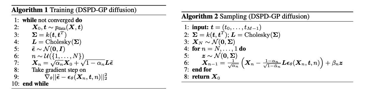
(2) Discrete stochastic process diffusion (DSPD)

Apply the discrete diffusion framework to the TS setting

• Discrete = number of diffusion steps

Notation

• \(\boldsymbol{X}_0\) : input data
• \(\boldsymbol{X}_n=\left(\boldsymbol{x}_n\left(t_0\right), \ldots, \boldsymbol{x}_n\left(t_{M-1}\right)\right)\) : noisy output after \(n\) diffusion steps

Comparison

• (DDPM) Adds independent Gaussian noise to data
• (Proposed) Add the noise from a stochastic process

Given the times of the observations, can compute the covariance \(\boldsymbol{\Sigma}\) and sample noise \(\boldsymbol{\epsilon}(\cdot)\)

( from GP or OU process )

• \(q\left(\boldsymbol{X}_n \mid \boldsymbol{X}_0\right) =\mathcal{N}\left(\sqrt{\bar{\alpha}_n} \boldsymbol{X}_0,\left(1-\bar{\alpha}_n\right) \boldsymbol{\Sigma}\right)\).

• \(q\left(\boldsymbol{X}_{n-1} \mid \boldsymbol{X}_n, \boldsymbol{X}_0\right) =\mathcal{N}\left(\tilde{\boldsymbol{\mu}}_n, \tilde{\beta}_n \boldsymbol{\Sigma}\right)\).

Generative model

= Reverse process \(p\left(\boldsymbol{X}_{n-1} \mid \boldsymbol{X}_n\right)=\mathcal{N}\left(\boldsymbol{\mu}_\theta\left(\boldsymbol{X}_n, \boldsymbol{t}, n\right), \beta_n \boldsymbol{\Sigma}\right)\),

• keeping the time-dependent covariance \(\boldsymbol{\Sigma}\).

Key difference

• Model now takes the full TS consisting of noisy observations \(\boldsymbol{X}_n\) with their timestamps \(t\) to predict the noise \(\epsilon\) ( which has the same size as \(\boldsymbol{X}_n\) )

Loss can be calculated in closed-form.

• can reparameterize the model s.t \(\boldsymbol{\Sigma}\) disappears from the final loss
• (Standard) \(\mathcal{L}=\mathbb{E}_{\boldsymbol{\epsilon}, n}\left[ \mid \mid \boldsymbol{\epsilon}_\theta\left(\sqrt{\bar{\alpha}_n} \boldsymbol{X}_0+\sqrt{1-\bar{\alpha}_n} \boldsymbol{\epsilon}, n\right)-\boldsymbol{\epsilon} \mid \mid _2^2\right]\)
• (Proposed) \(\mathcal{L}=\mathbb{E}_{\boldsymbol{\epsilon}, n}\left[ \mid \mid \boldsymbol{\epsilon}_\theta\left(\sqrt{\bar{\alpha}_n} \boldsymbol{X}_0+\sqrt{1-\bar{\alpha}_n} \boldsymbol{\epsilon}, \boldsymbol{t}, n\right)-\boldsymbol{\epsilon} \mid \mid _2^2\right]\)

Sampling

• initial noise
  • stochastic process (O)
  • independent normal distribution (X)

(3) Continuous stochastic process diffusion (CSPD)

( Apply it to Score-based SDE instead of DDPM )

Noise scales \(\beta(s)\)

• continuous in the diffusion time \(s\)

Factorized covariance matrix \(\boldsymbol{\Sigma}=\boldsymbol{L} \boldsymbol{L}^T\) …

VP-SDE : \(\mathrm{d} \boldsymbol{X}_s=-\frac{1}{2} \beta(s) \boldsymbol{X}_s \mathrm{~d} s+\sqrt{\beta(s)} \boldsymbol{L} \mathrm{d} W_s\).

\(\rightarrow\) Transition probability: \(q\left(\boldsymbol{X}_s \mid \boldsymbol{X}_0\right)=\mathcal{N}(\tilde{\boldsymbol{\mu}}, \tilde{\boldsymbol{\Sigma}})\)

• \(\tilde{\boldsymbol{\mu}} =\boldsymbol{X}_0 e^{-\frac{1}{2} \int_0^s \beta(s) \mathrm{d} s}\).

• \(\tilde{\boldsymbol{\Sigma}} =\boldsymbol{\Sigma}\left(1-e^{-\int_0^s \beta(s) \mathrm{d} s}\right)\).

Score function can be computed in closed-form

• \(\nabla_{\boldsymbol{X}_s} \log q\left(\boldsymbol{X}_s \mid \boldsymbol{X}_0\right)=-\tilde{\boldsymbol{\Sigma}}^{-1}\left(\boldsymbol{X}_s-\tilde{\boldsymbol{\mu}}\right)\).

\(\rightarrow\) Optimze \(\mathcal{L}=\mathbb{E}_{\boldsymbol{x}_s, s}\left[ \mid \mid \psi_{\boldsymbol{\theta}}\left(\boldsymbol{x}_s, s\right)-\nabla_{\boldsymbol{x}_s} \log p\left(\boldsymbol{x}_s\right) \mid \mid _2^2\right]\)

Summary: \(\boldsymbol{\epsilon}_\theta\left(\boldsymbol{X}_s, \boldsymbol{t}, s\right)\) will take in …

• (1) Full TS \(\boldsymbol{X}_s\)
• (2) Observation times \(\boldsymbol{t}\)
• (3) Diffusion time \(s\)

( Again use the reparameterization in which we predict the noise, whilst the score is only calculated when sampling new realizations. )

= That is, we represent the score as \(\boldsymbol{L} \tilde{\boldsymbol{\epsilon}} / \sigma^2\), where \(\sigma^2=1-\exp \left(-\int_0^s \beta(s) \mathrm{d} s\right)\)

• \(\tilde{\boldsymbol{\epsilon}}\) : Noise from Gaussian