Masked Diffusion Models are Fast Distribution Learners
Contents
- Abstract
- Introduction
-
Related work
- Masked Diffusion Models
- Intuition
- Masked Pretraining
- Model Architecture & Masking Configuriaton
- Efficiency
0. Abstract
Diffusion = significant training overhead
\(\rightarrow\) This paper shows that it sufficies to set up pretraining stage to initialize diffusion
\(\rightarrow\) Then perform finetuning for specific generation task
Pretraining: masking
- (1) Mask a high proportion (90%)
- (2) Employ masked denoising score matching
1. Introduction
Investigate if denosiing training can avoid modeling from raw image in the early trianaing stage
\(\rightarrow\) Enhancing the overall training efficiency!
Intuition: First, capture global structure !
( = Make training easier by first aapproximating some “primer” distns )
\(\rightarrow\) Subsequent modeling of detailed info can be accelerated
HOWEVER … how to learn such primer distributions ??
\(\rightarrow\) By “masked modeling”
- Define primer distribution as… Distn that shares same group of marginals
Propose Masked Diffusion Models (MaskDM)
Two stage of MaskDM
- Masked pre-training
- Mask input image
- Perform MDSM (Masked Denoising Score Matching)
- Denoising finetuning
- with conventional weighted DSM (Denoising Score Matching) objective
Plug-and-Play technique with existing models
2. Related Work
DSM loss:
\(L_{\text {simple }}(\theta)=\mathbb{E}_{t, \boldsymbol{x}_0, \epsilon}\left[ \mid \mid \boldsymbol{\epsilon}-\boldsymbol{\epsilon}_{\boldsymbol{\theta}}\left(\sqrt{\bar{\alpha}_t} \boldsymbol{x}_0+\sqrt{1-\bar{\alpha}_t} \boldsymbol{\epsilon}, t\right) \mid \mid ^2\right]\).
3. Masked Diffusion Models
(1) Intuition
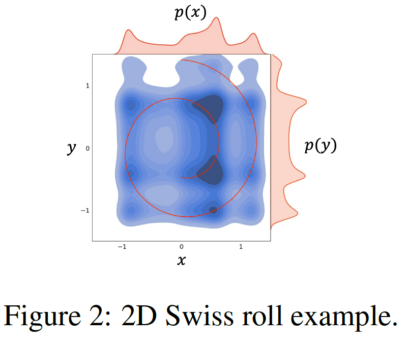
Notation
\(p(\boldsymbol{z})\) .
- GT 2D Swiss roll distribution (Red line)
- \(\boldsymbol{z}=(x, y)\).
\(p(\boldsymbol{z})\) .
\(p_\phi(\boldsymbol{z})\) .
- Model (Blue heatmap)
- Fully covers the target distribution \(p(\boldsymbol{z})\), t
Rather than approximating \(p(\boldsymbol{z})\) from scratch ….
\(\rightarrow\) gradually shaping a distribution initialized as \(p_\phi(\boldsymbol{z})\), which shares with \(p(\boldsymbol{z})\) the same MAGINAL distribution, i.e., \(p(x)\) and \(p(y)\), is expected to be comparably easier
Initializing a task for approximating a high-dim \(p(\boldsymbol{z})\) with \(p_\phi(\boldsymbol{z})\), which partially preserves the sophisticated relations between different marginal distributions, may bring even more computational benefits
- Masked image can be seen as a sample drawn from a marginal distribution that is identified by the selected square blocks, which marginalize out all covered pixels
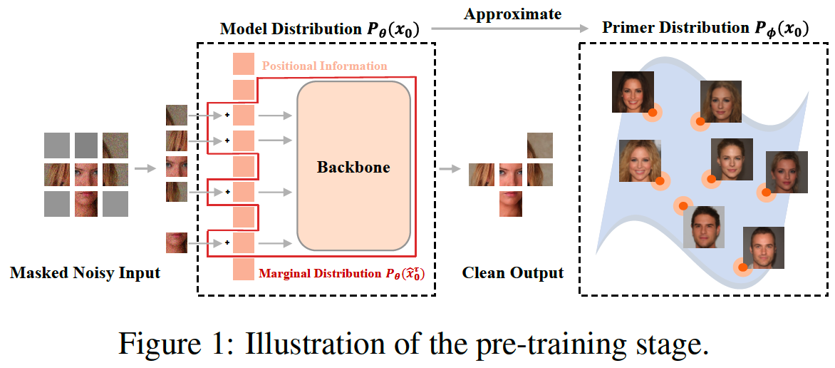
(1) Masked Pre-training
Image \(x_0\) = Vector: \(\left(x_0^1, x_0^2,, x_0^3, \ldots, x_0^N\right)\),
- where \(N\) represents the number of pixels
Data distribution \(p\left(\boldsymbol{x}_0\right)\)
- expressed as the joint distribution of \(N\) pixels.
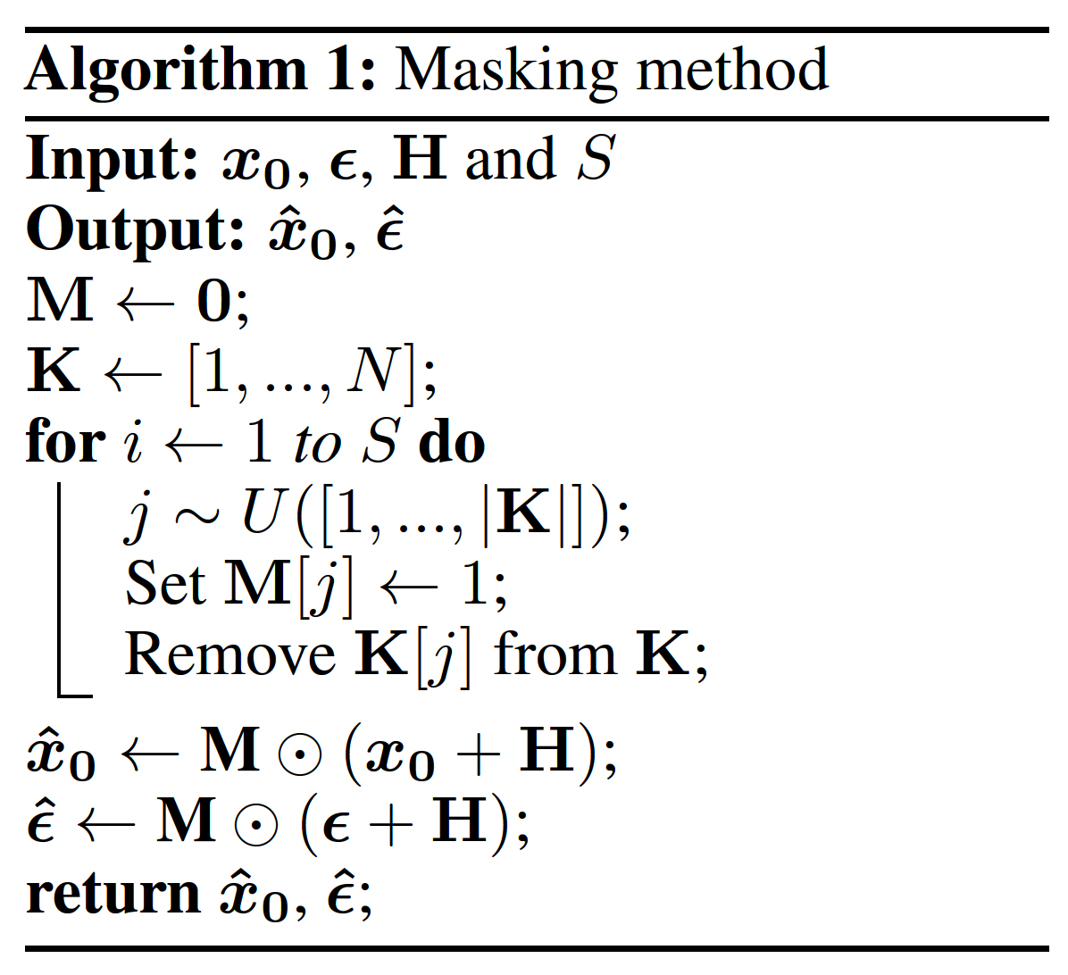
\(\tau\) : Randomly selected subsequence of \([1, \ldots, N]\) with a length of \(S\).
- Selected pixels = \(\left\{x_0^{\tau_i}\right\}_{i=1}^S\)
- Marginal distribution of them = \(p\left(\hat{\boldsymbol{x}}_{\mathbf{0}}^{\boldsymbol{\tau}}\right)=p\left(x_0^{\tau_1}, x_0^{\tau_2}, x_0^{\tau_3}, \ldots, x_0^{\tau_S}\right)\).
\(\hat{\boldsymbol{x}}_0\) = Any marginal variable combinations
-
\(\left\{\tau \in[1, \ldots, N], \mid \tau \mid =S \mid \hat{\boldsymbol{x}}_{\mathbf{0}}^\tau\right\}\),
-
\(p\left(\hat{\boldsymbol{x}}_{\mathbf{0}}\right)\) = corresponding marginal distn
\(p\left(\boldsymbol{x}_{\mathbf{0}}\right)\) belongs to \(\mathcal{Q}\)
- Family \(\mathcal{Q}\) of distributions = Share the same set of marginal distn \(p\left(\hat{\boldsymbol{x}}_{\mathbf{0}}\right)\).
Primer distribution \(p_\phi\left(\boldsymbol{x}_{\mathbf{0}}\right)\)
= Any distn in \(\mathcal{Q}\) other than \(p\left(\boldsymbol{x}_{\mathbf{0}}\right)\) that satisfies this condition
However, non-trivial to approximate \(p_\phi\left(\boldsymbol{x}_{\mathbf{0}}\right)\), particularly when the samples from \(p_\phi\left(\boldsymbol{x}_{\mathbf{0}}\right)\) are not available!!
\(\rightarrow\) Initialize the task ( = masked modeling ) of approximating \(p_\phi\left(\boldsymbol{x}_{\mathbf{0}}\right)\) with a diffusion model \(p_\theta\left(\boldsymbol{x}_{\mathbf{0}}\right)\),
-
In each training iteration, by training with a batch of images sampled from some arbitrary “marginal” distributions ( = sampled from \(p_\theta\left(\boldsymbol{x}_{\mathbf{0}}\right)\) ),
we are implicitly approximating \(p_\phi\left(\boldsymbol{x}_{\mathbf{0}}\right)\) by modeling all its “marginals”
Notation
-
Image input \(\boldsymbol{x}_{\mathbf{0}}\)
-
Additional inputs
- (1) Masking vector \(\mathbf{M} \in\{0,1\}^N\)
- (2) Positional information \(\mathbf{H} \in R^N\) of the visible pixels
( additional clues to distinguish different marginal distributions )
Simple masking approach suffices to …
- preserve meaningful visual details
- enabling a much faster pre-training convergence
- further facilitates subsequent fine-tuning
- \(\hat{\boldsymbol{x}}_{\boldsymbol{t}}=\sqrt{\bar{\alpha}_t} \hat{\boldsymbol{x}}_{\boldsymbol{0}}+\sqrt{1-\bar{\alpha}_t} \hat{\boldsymbol{\epsilon}}\).
- masked image \(\hat{\boldsymbol{x}}_{\boldsymbol{0}}\)
- noise \(\hat{\boldsymbol{\epsilon}}\)
- MDSM objective
- \(L_{m d s m}(\theta)=\mathbb{E}_{t, \hat{\boldsymbol{x}}_{\mathbf{0}}, \hat{\boldsymbol{\epsilon}}}\left[ \mid \mid \hat{\boldsymbol{\epsilon}}-\boldsymbol{\epsilon}_{\boldsymbol{\theta}}\left(\sqrt{\bar{\alpha}_t} \hat{\boldsymbol{x}}_{\mathbf{0}}+\sqrt{1-\bar{\alpha}_t} \hat{\boldsymbol{\epsilon}}, t\right) \mid \mid ^2\right]\).
(2) Model Architecture & Masking Configuration
Backbone = U-ViT
Configuriation of masking setting
-
(1) \(S\) (or the mask rate \(m=1-\frac{S}{N}\) )
-
\(m\) determines the average degree of similarity between the true data distribution and the primer distributions
( such that a lower value of \(m\) indicates a greater resemblance )
-
-
(2) Strategy for sampling the mask vector \(\mathbf{M}\)
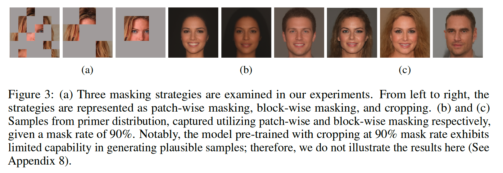
Three different masking strategies
- (1) Patch-wise masking
- (2) Block-wise masking
- (3) Cropping
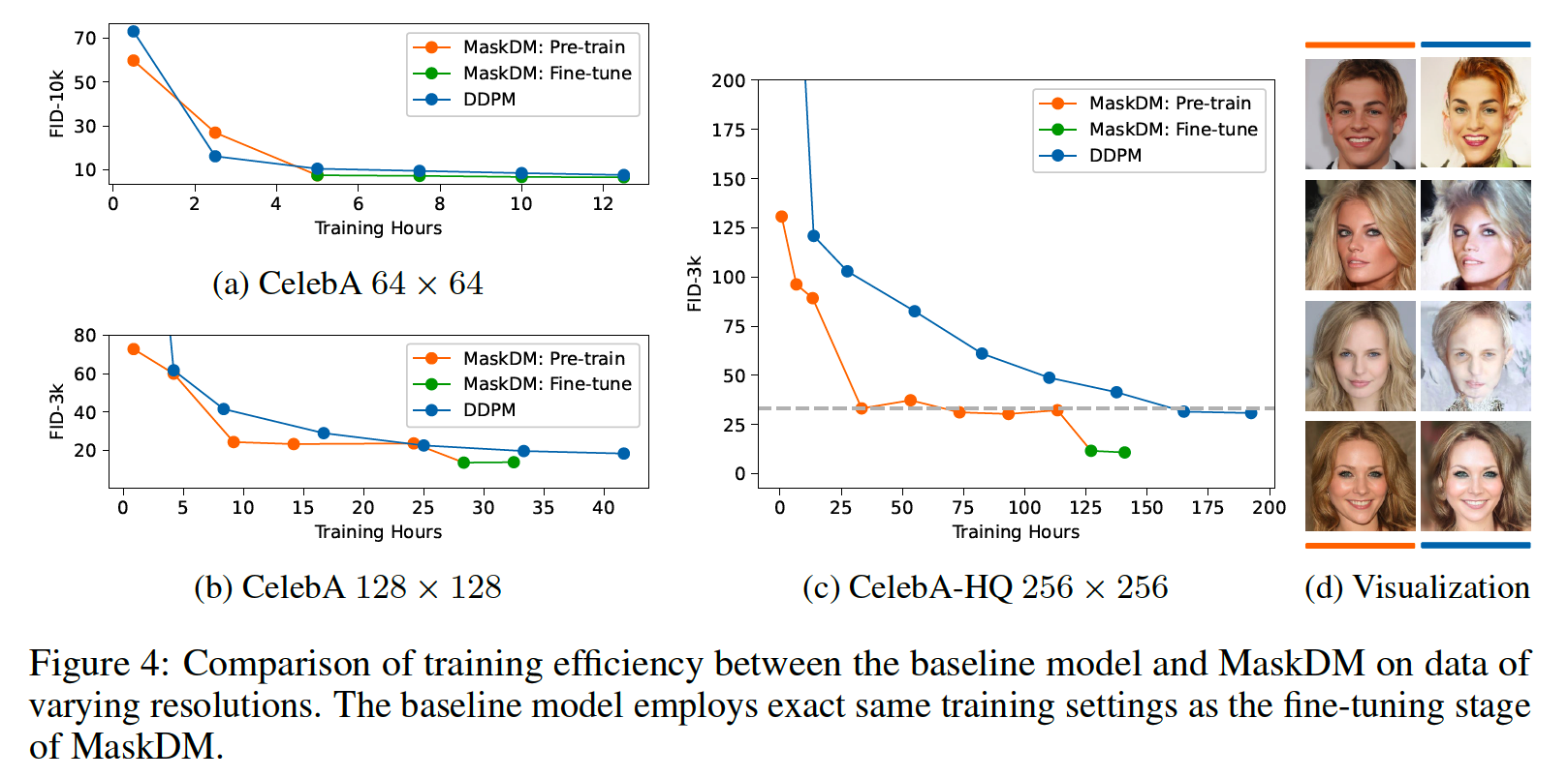
4. Efficiency